Tactical Sailing

Marika is an avid sailor, and former Fleet Captain of the University of Michigan Sailing Club. In hearing about her exploits on the high seas (or Huron River, as the case may be), I've often thought about the mechanics of sailing. Specifically, I was curious if I could model the forces involved in maneuvers like tacking and jibing.

The model I came up with was to consider two connected forces on the boat: wind hitting the sail, and drag from the water. When wind hits the sail, the air bounces off, imparting momentum in the direction of the surface of the sail. The magnitude of the momentum transferred will be proportional to the dot product of the sail direction and the wind direction – maximum is when the wind hits the full face and zero when it's perpendicular. The drag from the water will be similar to the wind hitting the sail, but this time we're looking at the shape of the hull for each bit of water that hits the boat. Both these forces depend on and change the velocity of the boat, so we iterate the calculation until we find the equilibrium. To do that, we need to come up with a model for the hull of the boat.

I couldn't find any existing mathematical models for hull shape, but looking at common designs, I came up with this concept: Take two halves of an ellipse with semi-axes a and b, and put them a distance W apart. As long as W is less than 2a, the halves will intersect at each end. Now measure L from one end, and cut the remainder off. Using numbers for the width and length from here, and picking a and b that seemed reasonable, here's what I came up with:

Now to the simulation: We consider a wind going from left to right and try different orientations of the boat and sail. For each case, we start with zero velocity and calculate forces from wind and drag. Those forces give a new velocity, and we repeat until there's little change. The final velocity is shown by the arrow. Now, I didn't want to spend a lot of time figuring out the exact momentum transfer for the wind and drag, so I fudged the scaling to get reasonable results. Even with this super simple model though, we can see cases where it's possible to sail into the wind! (Look for the arrow pointing left.)

As with all of my posts, I don't recommend trying this yourself based on my calculations, but I'm hoping Marika will give me some experimental experience in the future!

In My Corner

For a while I've been interested in analyzing the game Jenga, since it's very physics-aligned in its design: Maintaining balance under changing forces. I couldn't get a handle on how to look at it though, until I connected it to a tool that's used frequently in my research field: corner plots. Corner plots are a way to display correlations between different variables in a large data set. For gravitational waves, they're used to show how estimates of a source's parameters depend on each other, such as a black hole's mass and spin. I figured I could come up with some measurements of Jenga games, and look at how they relate to each other.

First, we need a way to collect some data. As a reminder, here's what a Jenga tower looks like:

Wikipedia

Each level has 3 blocks that alternate in direction. On a turn, we remove a block from anywhere below the top level, and then add it to the top. The tower will fall and end the game if the center of mass of a subset is over an empty space, and the side is not supported. I was able to make a simulation of this in Python, with the virtual player making a random move on each turn, so long as that move does not cause the tower to fall. Eventually, the player will run out of moves and the game will end, but we can look at what kinds of moves result in longer games. I struggled a bit to find a way to show an example tower being built, and settled on a side view with all the bricks facing out. Remember that the bricks actually alternate in direction, so a hole under a brick is not necessarily a problem:

Now to get our statistics, we want to run a large series of games, and get some measurements from each one. The parameters I chose were max height of the tower, number of turns taken, fraction of turns for which the center block of a level was removed, fraction of turns a block was placed on the center of the top, and the fraction of times a block was removed from the upper half of the tower. After running 500 simulated games, we can make a corner plot with the results (click to enlarge):

This shows us some interesting connections between our parameters. There is strong correlation between the maximum height and the number of turns – This makes sense, since each turn we put a brick on the top level. We can also see anti-correlation (negative slope) between removing the center brick and max turns/height. This is because once the center of a level is taken, we can't take either of the sides, so we run out of bricks faster. Our final two variables, adding to the center and removing from the upper half, don't seem to have much effect on the outcome, indicated by the circular distributions.

Now in reality, Jenga bricks are designed with some irregularities to make the balance a little more difficult to predict, so this is another case where knowing the physics might not help you win, but it was interesting way to explore a tool for visualizing data.

Rings a Bell

A couple weeks ago, it was announced that this year's Nobel Prize in Physics was going to a group of scientists who experimentally tested Bell's Theorem. As with many concepts in quantum mechanics, this can be a bit tricky to understand, so I wanted to build it up piece by piece (as much for myself as for you).

When Quantum Mechanics was first developed, many people (including Einstein) were disturbed by the implication that, not only did interactions have random results, but that entangled particles could communicate those results instantaneously, breaking the speed of light. One explanation that was proposed to avoid this problem was the "Hidden Variable Hypothesis", which claimed the final states of the entangled particles were actually determined by some unknown property present at their joint creation, and therefore no information needed to be exchanged. John Bell came up with a way to test for the presence of a hidden variable, which I'll outline below.

First, suppose we have some collection of measurements. Each measurement has three properties: A, B, and C, which can either be +1 or -1. If each property is assigned randomly, we can think about the probability of two properties being the same, e.g. P(A = B). Now we can write

If you're not sure about this, you can try a couple sets of values, but the key is that we only have 2 choices, +1 and -1, for 3 properties. Now these properties are exactly the type of hidden variables that we're suggesting may exist. If we can come up with an experiment that can measure yes/no for three different properties, then we can simply count the outcomes and check if this inequality holds.

Looking again at that old post I linked to, we can imagine the following experiment: We produce entangled particles with opposite spin, and send them in opposite directions. Each goes into a Stern-Gerlach box and gets measured as spin-up or spin-down on the box's axis. However, we vary the angle of each box between 3 possibilities: 0°, 120°, and 240°. Our three properties are "spin-up along n-degree axis", and negation represents spin-down.

With this setup, we can think of the hidden variables as a set of rules for how the particles respond to each of the three angles. When a pair is produced, each is assigned one of these rule sets, e.g.

Since the particles have opposite spin, comparing the two detectors means the equalities in the equation above become not-equal. Now we can look at all the possible combinations of A, B, C between the two detectors, as well as each set of rules the pairs could be assigned, and find the probability that the two measurements are opposite:

In the inequality above, each term contributes 1/3, which gives us a total of 1 and satisfies the relation.

Quantum mechanics, though, predicts a different result. When one of the entangled particles is measured to be spin-up along a particular axis, we immediately know the other one is spin-down along that same axis. Knowing the second particle's orientation, we can find the probabilities of measuring opposite spin along each of the possible axes:

Adding up the terms again, according to Quantum Mechanics we only get 3/4, violating Bell's Inequality! That means we have an experimental method to test for hidden variables. Unfortunately, dealing with entangled particles is a delicate process, and the experiment needs to be repeated several times to accurately measure the statistical distributions, which is why it has taken more than 50 years to confirm this result. A well-deserved Nobel Prize for these scientists!

A Churning Ring of Water

[Title with apologies to Johnny Cash.]

The sink in our new home has an interesting setting that I was curious about:

It sprays a thin film outward, but the water curves back to meet in the middle again. When the water leaves the sprayer, there are only two forces acting on it: gravity pulling it down, and surface tension pulling the droplets together. I mentioned surface tension long ago, but I've never dug into the mechanics of it.

Surface tension is a force that acts to decrease the surface area of a fluid. For a given volume, a sphere has the smallest surface area, which is why water forms drops, and why shot towers can make round bullets. The magnitude of the force is given as

where γ is a constant that depends on the two materials being considered (air and water in this case) and L is the length of the edge that F will act to reduce. The sink is spraying out a ring of water, so if we take a cross-section, L is the inner plus the outer circumference of the ring. We can rewrite the force as

where m is the total mass of water, a is the acceleration, ρ is the density, A is the area of the ring, and Δh is the small vertical slice we're considering. Now this a refers to the radial acceleration of each water molecule, but we want to relate it to back to L. To do that, we can write two equations expressing L and A in terms of the inner and outer radii of the ring:

Since the ring is thin, we can take r1 approximately equal to r2, and after a bunch of algebra write

Since the flow of water is constant, A must be constant, so we can use the above equation to get a timeseries for L, then find r1 and r2.

In order to integrate this, we need initial values for L and Ldot. We can approximate the opening on the faucet to get r1 and r2, and find the initial L and the constant A. Then we can use A with the typical flow rate of 2.2 gallons/minute to find Ldot. Something didn't quite work out with my estimations, since the scale is way off in the following plots, but the shape matches great. Here's a side view of the spray:

and an animation descending through cross-sections:

So far I haven't found much use for this setting when cleaning dishes, but it did give me something interesting to think about!

A Charge of Battery

This week, I have a question from my mother Sally about their Chevy Bolt: I was thinking about the most efficient way to drive the Bolt on a long trip: Do you drive more slowly, so that your miles/kWh are more and you don’t need to charge as much? When you do charge do you stop frequently and only charge at the highest rate (the rate declines as the battery % is higher, e.g. 42kWh, declining to 26kWh), or do you stop as little as possible and stay until you’re at 80%?

As Sally outlines, there are two states the car will be in during a trip: charging and driving. The amount of time it takes to add a certain amount of charge to the battery depends on how much charge is in it – As it fills up, it gets harder to add more. During charging then, we can write

that is, the rate of charging is proportional to the space remaining. While driving, we have to push against a wind resistance that depends on our speed:

Drag typically depends on the square of velocity, meaning that increasing speed can quickly become counter-productive.

Now, both these equations I've written are just proportionalities, which need specific scales and shapes. Normally I'd have to make up something based on wild assumptions of a clueless physicist, but lucky for me, Bolt drivers are my kind of crazy, and have measured the behavior of their cars in detail!

For the first equation, I found this chart from InsideEVs:

and for the second, I found one from ChevyBolt.org:

Since these are just graphs, I had to do a bit of fitting, but I'm pretty happy with the results. To answer Sally's question, I chose a bunch of different driving speeds and max/min charge levels. We drive the car at the given speed until the battery hits the minimum charge level, then we stop and charge until it gets to the maximum charge. We continue for 1000 miles, then check the average speed during the trip, and the number of stops.

First, I plotted a heatmap of the average speeds for the different max/min charge values, planning to mark the point where we get the best speed and the fewest stops. Unfortunately, it turned out both of those always occurred with a min charge of zero, so it's easier to see them as lines:

I found this a bit difficult to take in, so I tried plotting only the zero min charge case for each speed:

This shows some really interesting results: Because of the difficulty in getting up to the battery's capacity, high max charge can result in spending most of your time charging, even at high speeds. However, if your max charge is too low, you have to stop over and over, even if it's only for short time.

Thanks for a great question, Sally!

A Parallax to Grind

Marika and I have an Apple TV, and if we leave it paused for a while, it goes into a screensaver panning over various scenes. One of these caught my eye, a view of the Isle of Skye in Scotland. If you skip near the end, you'll see an interesting effect where two pieces of land are moving by at different speeds, even though the camera is moving at a constant speed. This is due to the parallax effect, and I was curious what I could learn from their movement, similar to my earlier post on the angle of the Moon.

When light hits our eye, our brains translate the angle the light enters into a position. The angle of an object at x horizontal to our eye, and a distance d away will appear at an angle off center of

If we move horizontally, we change x, so for a constant velocity v the angle will change by

What this means is that even for the same camera position and speed, two objects will have different angular velocities based on their distance. We can visualize this with an animated plot:

On the left, we have the top-down view, where we see two objects moving past the camera at the bottom. On the right is the camera's view, where we can see that even though the blue begins ahead of the red, as we pass the objects, the closer red one races ahead. We can try to relate their speeds by using the equation for theta's change twice: the velocity and horizontal positions are the same for both, but the distances are different. Putting the two equations together gives

which says that if we take measurements at a few different horizontal positions, we'll be able to find a ratio between the distances, but not their individual values.

You may have noticed earlier I specified a single eye – Because we have two eyes, our brains can use this process without needing to move to find relative distances. This method also connects to astronomy: One way to measure the distance to a star is to observe it at different points in the Earth's revolution around the Sun – A planet-sized pair of binoculars!

Art is not My Fourier

A while ago, I saw this interesting video about Fourier series, a mathematical tool often used in physics. What really caught my attention was the demonstration of using the series to draw a picture, and how the picture changes as the number of terms increases. I was curious if I could come up with a way to apply this to any given picture.

Before getting into that though, I should give an idea of what a Fourier series is. If you have 25 minutes, the video above is really great, but basically a Fourier series allows us to express a periodic function as a sum of all the different frequencies involved. Here's a nice example from Wikipedia showing an approximation of a square wave using the first 6 terms of the Fourier series:

Wikipedia

We can extend this idea to 2 dimensions using the complex Fourier series. This replaces sine and cosine with the complex exponential. Again, if you want more details, I highly recommend the video above. What it boils down to is that we draw our image with the sum of a bunch of arrows, each rotating at a fixed rate.

Since we need a periodic function in order to make a (finite) Fourier series, we need to use an image that consists of a single unbroken curve. In the video, the examples are all simple line drawings, but I hoped to find a way to convert an image to such a curve automatically. Lucky for me, such algorithms have been developed for use with CNC machines and laser engravers. These require a path for the tool to follow to trace out an image. I found some Python code that accomplishes this by finding the edges of shapes and linking them into paths.

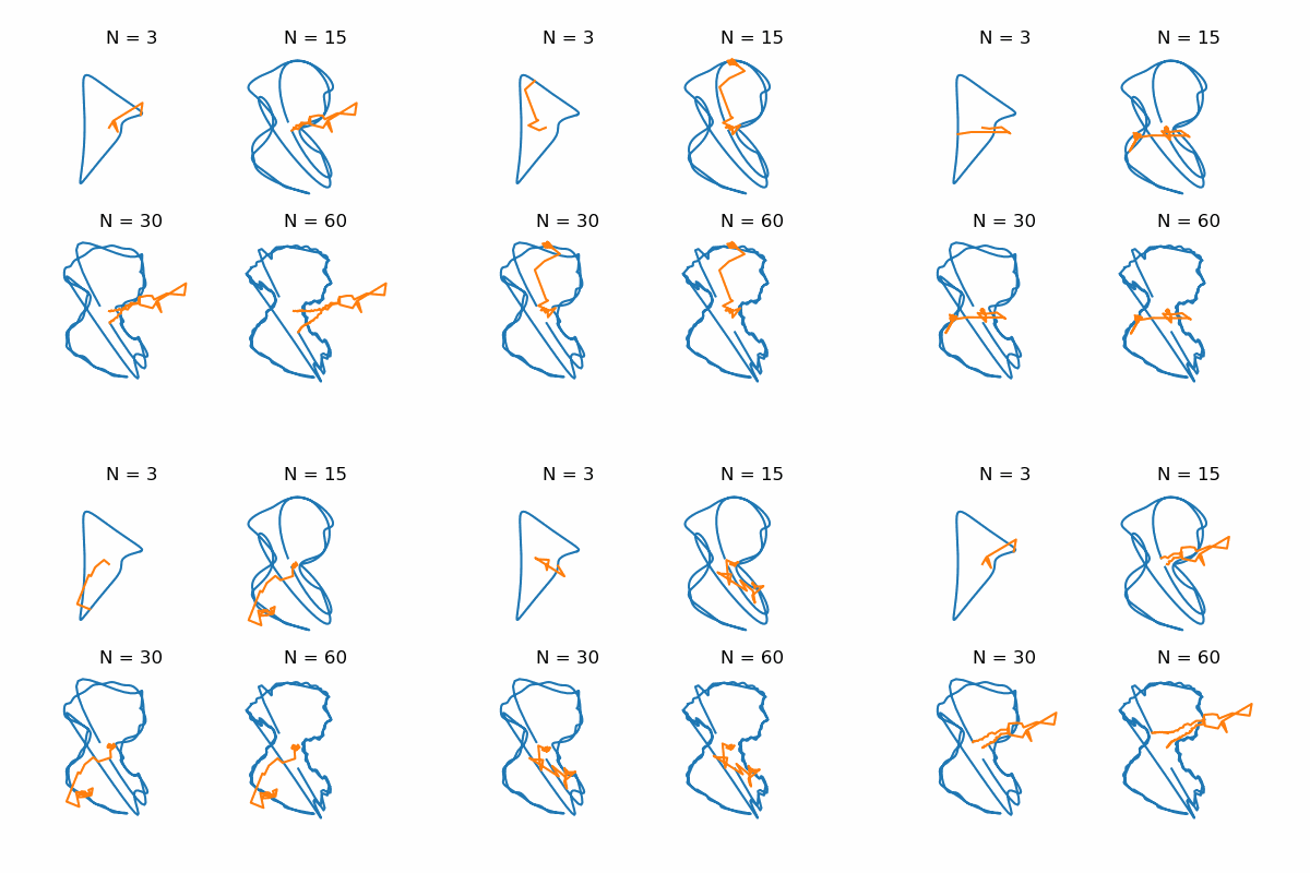
The specific question I was curious about was how the image changes depending on the number of terms. With only a single term, for example, we'd just draw a circle. As the number increases, we get more of the fine details. You can try the code yourself here – I found simple images work best. Photo quality images tend to have too much shading, which doesn't lend itself to reducing the number of terms.

As a first try, I drew a simple smiley, on the principle that it's mostly circles:

The orange lines show each rotating arrow. Pretty quickly the outer circle asserts itself, but the small eyes take some time to appear. After a bit of experimentation with different images, I realized the ideal case for my method was a silhouette. Here's one of an airplane using the same orders of terms:

Based on Wikipedia

Of course, when we talk about silhouettes, we usually imagine people, so here's one I found of Jane Austen:

Based on Wikipedia

It's interesting how the pointier bits of her profile move around: First nose, then bun. This is another of those post ideas that's been lying around for a while since I assumed it would be prohibitively difficult, but once I found that line tracing code it was a snap! I hope if you find this interesting you'll give it a try, and share the results.

Self-Jamming Cars

This week I wanted to try another Complex Systems-style simulation, this time based on something I had originally seen on Mythbusters, but others have tried with similar results: Traffic jams that appear out of nowhere simply due to drivers varying their speed. The system is fairly simple: Some number of cars drive on a circular track, trying to go as fast as possible while maintaining a safe stopping distance and obeying the speed limit. However, they may not all accelerate at the same speed, and can brake unexpectedly. These error factors result in some interesting effects, including waves of slow speed that travel backwards around the track.

To simplify things, I assumed the cars were either accelerating at maximum, or braking at maximum. They would decide based on the stopping distance from the car ahead of them:

where v is the car's velocity, and a_b is the braking acceleration. If the distance to the next car is less than this, we brake, otherwise we continue accelerating.

The controls you'll find below are the number of cars on the track, the maximum speed they'll go, the rate of acceleration, the rate of braking, the size of the variation in acceleration rate, and the rate at which that variation changes. This last factor is needed because if we change the acceleration error at every step, it tends to average out and have little effect. There's also a brake button that makes the red car slow while holding it down. As with many of these Complex Systems topics, I'm always surprised by the dynamics that emerge with just a few simple rules. Be sure to post a comment if you find something particularly weird!

Dreamt of in Your Philosophy

This week, I got several questions from Papou about the Big Bang and thermodynamics:

Is the Universe a closed system?

In order to answer this, we need to define what is meant by a "closed system": This is where no matter or energy enters or leaves the system under consideration. That means that the Earth, which gets energy from the Sun and radiates it back into space, is not a closed system. The Universe, however, which contains all matter and energy observed, is a closed system.

A different question, which uses confusingly similar terms, is whether the Universe is open or closed in the geometric sense. This refers to what happens if you travel in a straight line: Do you eventually come back to where you started, like you would on the surface of the Earth? Due to the influence of dark energy, for our universe the answer is no, it is geometrically open, whatever Modest Mouse may tell you.

How do the Laws of Thermodynamics apply to the Big Bang Theory?

Before we dive into this, let's talk about what the laws of thermodynamics are:

1. The energy in a closed system remains constant.
2. In any process, the entropy of the system must increase or stay the same.
3. As temperature approaches absolute zero, entropy approaches a constant

These are sometimes summarized as

1. You can't win.
2. You must lose.
3. You have to play the game.

I've mentioned entropy a couple of times on this blog, each time in a slightly different context. In this case, it can be thought of as energy that can no longer be used for work. As an example, if you have a bottle of compressed air, you could use it to propel a cart or turn a pinwheel, but if everything's at the same pressure, the air won't flow. This is actually the plot of a short story I read recently called Exhalation, about robots powered by compressed gas.

The Big Bang theory states that all matter and energy in the Universe started at a single point, which expanded outward. We can check off the first law, since the theory isn't saying anything about where that point came from – The Universe started with some fixed energy, and that energy is still here, just more spread out. That last part applies to laws 2 and 3 – Spreading out means more possible states for the matter, and lower temperature. It's these laws that lead to the heat death of the Universe, which I described before.

What is the impact of the Laws of Thermodynamics on Evolution?

The laws I outlined above are sometimes used as an argument against evolution: Evolution makes things more ordered, but that violates the increasing entropy requirement. The key is that the second law doesn't say entropy everywhere increases, just that it increases in the system as a whole. It's true that a human body has less entropy than a pile of microbes of the same mass, but that skips all the entropy generated in producing a human body. For a (slightly) more detailed discussion, I found this page, written by Robert Oerter at George Mason University.

Can there ever be enough Hawking Radiation to eliminate a Black Hole?

Yes! Hawking radiation is a process by which black holes can emit particles, but according to the first law up above, that means the black hole must lose energy/mass. If this happens over enough time, or the black hole is small enough, it can eventually evaporate. When the Large Hadron Collider first started up, some people (not scientists) were afraid it would create a black hole that would swallow the Earth. Experts were confident that if it did create one of the hypothesized microscopic black holes, they would quickly evaporate under Hawking radiation.

Thanks for more great questions, Papou!

Candlemass

On a camping trip a little while ago, I was watching the wood shift in the fire, and I came up with an interesting thought experiment: If you put a candle on a scale and light it, what does the scale read over time? Obviously over a long time, the measured weight will decrease, since the candle is burning away, but for a short time after lighting, would the weight appear to go up from the mass being ejected from the candle?

The candle is throwing gasses upward at some velocity, giving them momentum. This in turn pushes the candle down with the same change in momentum, similar to how a rocket works. Change in momentum is the same as a force, and we also have gravity pushing down according to the current mass:

To calculate the momentum change, I decided to use the average speed of an ideal gas:

Where k is Boltzmann's constant, T is the temperature in Kelvin, and m is the mass of the molecule. When things burn, they typically give off two types of molecules: water, and carbon dioxide. To figure out how much, we'll need to do a bit of chemistry. Candle wax is typically a large hydrocarbon, which combines with oxygen:

For beeswax, n is 45, so since I'm a physicist, I'm going to call that big and throw out those plus-2s to say that for every 1 unit of carbon burned, there are 2 units of hydrogen and 3 of oxygen. Now we can write the total change in force as 

The Wikipedia article I linked above gives a burn rate of about 0.1 g/minute. Plugging in a couple different temperatures, we can plot this function over a few minutes:

Impressively, the candle will register a greater force on the scale for around 8 minutes! Less impressively, that extra force will be around 2 thousandths of a pound. Looks like Yankee Candle won't be starting a space program anytime soon.

The Great Mubbet Caber

I may have mentioned before that I'm a big fan of the British quiz show QI. A recent episode included a discussion of an event from the Scottish Highland Games, the caber toss. In the sport, competitors must throw what amounts to a tree trunk such that it flips end-over-end and lands pointing as straight as possible away from them. You can see a video with some examples here:

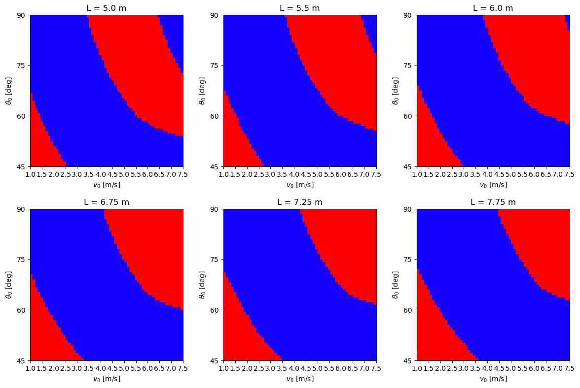
I was really curious about the physics involved in determining a successful flip. I decided to make a simplified model of the sport: The competitor holds the caber at an initial angle θ, measured from the horizontal behind them. Then they run forward up to a speed v, and stop, exerting a torque on the end of the caber. It continues forward, while beginning to spin. When one end touches the ground, it sticks, and then the initial speed and gravity determine which direction it falls.

Based on the Wikipedia article I linked above, I tried a range of different lengths (5-7.75 m), angles (45-90°), and initial velocities (1-7.5 m/s or 2-17 mph). For each case, I ran the simulation and tested whether the caber fell away, or back toward the athlete. The plots below show the results, with blue indicating success, and red failure. As the length changes, the successful ranges shift, and for the shortest cabers they can even flip twice (blue region in the upper right)!

For the longest case, I also animated the throws for the 4 corners: min/max speed and angles:

As with many of these posts, I'm not sure understanding the theory would make me any more able to compete, but I'm content to use my imagination!

You Remind Me of the Babe

Recently, I was reminded of a toy my grandparents had when I was growing up, a marble maze like this one:

Amazon

Turning the knobs tilts the board, causing the marble to roll. I was curious if I could find the fastest possible path through the maze. The key is that the tilt of the board limits how much acceleration you can apply, which in turn limits the speed with which the ball can navigate turns.

Since hitting walls would introduce sharp changes in velocity, which makes things difficult to optimize, I decided to simplify the problem by leaving out the holes, and penalizing any path that passes through a wall – With a high enough penalty, the optimum solution should not allow any Kool-Aid balls.

The first problem to solve is representing the maze, and a path through it. I found a Python package that handles both of these, pyamaze. This package can generate a maze on a grid of squares, and give the series of points leading from the start to the finish. To go from these points to a continuous path, I decided to use spline curves. These are a technique for generating a function that passes smoothly through a given set of control points. By moving each control point around inside its square, we can try to find the fastest way to navigate the maze. Here's an example, using the initial centered points:

The spline curves are parameterized by a variable, which we'll call λ. This is defined such that each integer corresponds to one of the control points. This variable may not obey our acceleration limits, when going around a sharp turn for example. We can imagine a function λ(t), then use the chain rule to write a relationship between our spline curves, and the acceleration of the ball:

This is for the horizontal motion of the ball, and we can write a similar equation for the vertical motion. I struggled for a while with how best to derive the λ equation from these, and settled on the simpler solution of setting d^2λ/dt^2 = 0. This means λ increases linearly with time, at a constant rate given by

where a_max is the maximum acceleration applied by gravity.

Now we have a method to get the time associated with a given path – It remains to find a path with the shortest time. Each control point is an input, which means this problem has a high number of dimensions. We also need to keep each point inside its square, meaning this is a constrained problem. Both of these qualities make it difficult to optimize. I decided to use Scipy's dual annealing method, which gave good results. I may talk about annealing in a future post, since it's an interesting topic (which you may have more experience with than you expect).

In the animation below, I show the steps of the optimization. At each step, the algorithm adjusts the positions of the control points to minimize the total time, shown at the top.

Notice that as the optimization progresses, the path gets more straight lines, which allow the ball to accelerate without the speed limits imposed by tight curves. You can see this effect if we animate the ball's path in time:

We can check we're obeying the acceleration limits by plotting the value of the equation given above:

There appears to be some numeric error I couldn't get rid of that makes us cross the limits I set a little bit, but overall it looks like the best strategy involves whipping the knobs from one extreme to the other, suggesting this is another game where spastic movements are key!

Fusebox

I've been stuck for several weeks on an idea for a post, as well as doing some family visiting, so I've haven't been here for a while, but during one of those visits, I got another great question from Papou (paraphrased): I've been reading about plans for fusion power plants. How do they work?

Fusion is a type of nuclear power, but unlike the typical fission plants in use today, does not require radioactive elements such as uranium. In a fission reaction, the fuel naturally releases particles which heat the surrounding material, as well as knocking more particles off other parts of the fuel. Fission power relies on the natural release of neutrons from the fuel to spur further reactions. However, fission results in nuclear waste – radioactive materials not strong enough to supply power, but still dangerous to living things.

Fusion works along the opposite path: Forcing two atoms together until they bond, which releases energy. This is made difficult by the structure of an atom: protons and neutrons are bound together by the strong nuclear force in the atom's nucleus, which is surrounded by a cloud of electrons held by the electric Coulomb force. When we try to force two atoms together, initially the Coulomb force between their electrons will resist, until they get close enough for the strong nuclear force to pull the nuclei together.

To put some numbers to this idea, we can look at the potential energies of the two forces involved. The Coulomb potential is given by

where the first term is some constants, the qs are the charges of the two particles, and r is the distance between them. The nuclear potential is a bit more complicated, and requires making some approximations. I used the Reid potential, which uses terms of the form exp(-m*r)/m*r. We can look at how these two potentials behave near the nucleus:

The x-axis is measured in femptometers, or 10^-15 m, about the size of a proton. Notice that the Reid energy has a large dip at around that size. This dip is enough to make up for the rising Coulomb energy, and it's what makes fusion power an attractive energy source. The trouble is that at larger distances, the Coulomb force pushes the atoms apart. We can look at the point where the forces cancel:

You can read a potential energy plot like an elevation map: Objects go downhill, faster for steeper slopes. Anywhere flat, an object will stay still, but if it's the top of a hill, like above, it's an unstable equilibrium and will fall one direction or the other with a slight disturbance. Here, you can see that the crossing point appears between 5 and 6 fm. Getting atoms that close is extremely difficult, and a major obstacle to fusion power.

One way to do it is by heating and compressing the material. This is how stars like our Sun achieve fusion: Gravity squeezes the hydrogen into a tight area, increasing both the temperature, and the chances of atoms hitting each other. The fusion then releases more heat, continuing the process. To scale that down to a power plant though, we need a different way to squeeze the atoms together.

The solution to that is to create a plasma. By heating the hydrogen to a little over 150,000 °C, we can make it ionize, or separate into individual protons and electrons. That makes it susceptible to electric and magnetic fields, which we can use to compress it. This is the method used by tokamak reactors, including the ITER, which is set to be the biggest such reactor beginning operation in 2025.

The problem such reactors need to overcome for power generation is that heating the hydrogen into the plasma state, and containing it with the electromagnetic fields requires a significant input of power. If everything works correctly, the output from the fusion can surpass that, but so far the best we've been able to do is generating 70% of the input power, a net loss. The plan for ITER predicts it will achieve a 10-fold increase in generated power over the input. It's exciting to see the progress being made in this field, but we should keep in mind the tangible results may still be a long way off. Thanks for another great question, Papou!

Sidebandits

This week was another LIGO-Virgo-KAGRA collaboration meeting, and since my work has focused on the detector itself, I tried to attend more of the sessions on instrumentation than I did in my data analysis days. One topic that stuck in my head was a technique for sensing the sizes of the various optical cavities used in the detectors, sidebands. By modulating the frequency of the main laser beam, we can effectively create frequencies on either side of the central one. This is the inverse of the effect I discussed way back in my PhD work.

"Modulation" simply means we're multiplying two sinusoids together, and we can apply a trigonometry identity to turn that into a sum:

This says that the frequency of the modulated signal is the sum and difference of the two frequencies that went into it. Often we add this modulated signal back to the carrier, z_1. Then we have three evenly spaced frequencies: f_1-f_2, f_1, and f_1+f_2, hence the name "sidebands". What's interesting is the variety of shapes you can get from this simple setup.

As a way to help me get my head around how everything interacts, I put together another doodad (two in a row!) which you can play with below. The top plot shows the timeseries of the signal, and the bottom plot shows the real part of the Fourier transform, a representation of the relative sizes frequency components. You can control whether we add the carrier to the modulated signal with the checkbox. I realize this is a somewhat obscure topic (and certainly not "everyday") but I hope it's fun to play with even if you're not as crazy as me!

Snow Fugitive

A couple weeks ago I got a really interesting question/story from my friend Garrett, relating an experience entirely foreign to me here in Florida:

Last weekend we got a huge blizzard in MA. In Boston we tied the record for the most snowfall in a single 24h period (~24''). I have street parking and my car gets absolutely buried. Snow up to the windows on both sides. The next day I dig out and am driving my car. Everything is fine until I get on the highway. Once I am above ~50mph, my car starts to shake violently. I pull over, thinking I may have a flat tire. Nope. The tires are fine and no snow is in the wheel wells. So I drive again and it is still happening. So I come up with the following hypothesis: When my car was parked and getting snowed in, the snow built up more-so on the lower side of my wheels/rims. This gave my wheels an uneven moment of inertia. Below a certain speed the force and oscillation period of the unbalanced wheels was low. But above ~50mph my suspension could no longer compensate, and I began to feel the vibration (similar to an unbalanced washing machine).

My initial thought was that at a certain speed he was hitting the resonant frequency of the snow/wheel combination. As the wheel turns, it has to exert a centripetal force on the snow to keep it moving with the wheel. According to Newton, that means the snow is exerting a centrifugal force on the wheel, which will be given by

where m_s is the mass of the snow, v is the car's speed, R is the radius of the tire, and r is the direction from the wheel hub to the snow. This will be a sinusoidal force, with frequency proportional to the speed of the car. That appears to be consistent with Garrett's experience, where the vibration didn't start until he got to a certain speed.

To check that, we need to come up with a model of the car's suspension. I found this paper promising: It suggests a setup where the tire and the car suspension each act as a damped spring.

The ks are the spring constants, the cs are the damping coefficients, and the zs are the height from the road. We can write the forces on the wheel and body as

Each of these springs will exhibit resonance at a frequency we can calculate:

However, if we plug in some of the values used in the paper above, we get frequencies that correspond to about 1 mph or less! Garrett pointed out that I shouldn't be so surprised:

I think it makes sense that the resonance peak you identified is at such a low speed. I'm assuming that car manufacturers design the suspension to NOT resonate (due to unbalanced wheels) at typical driving speeds. Moreover, what I experienced did not feel like a resonance peak. I did not notice the vibration at all until I was above ~40mph or so, but from then on the vibrations increased with increasing speed. There was no point at which I felt the vibrations decrease as I increased speed. 

Taking another look at the equation for the snow's centrifugal force, we see it's proportional to v^2, so the faster the car is moving, the more the snow unbalances the wheel.

I put together a simulation of the system (using SSMs again, since I've been spending too much time around engineers) and we can see exactly this effect in both the average displacement of the car body:

and in the maximum displacement:

I had such a great time thinking about this and discussing with Garrett, I decided to put together another HTML5 doodad that you can play with below. I had to tweak the parameters a little, and there are still some significant transient effects, so you may get some crazy results just after changing the inputs, but they'll settle down after a few seconds. Thanks for the idea, Garrett!