Gaussamer Threads

At my lab's group meeting this week, one of my colleagues was showing off the tungsten cube he had purchased to be used in a satellite designed to measure the Earth's mass distribution, similar to the GRACE mission I discussed earlier.

(May contain Infinity Stone)

Since we want the cube to be only affected by gravity, one of the steps in fabrication is degaussing, or removing any residual magnetism. I was curious about this process, since it didn't align with my previous context for degaussing: In high school, I worked for the IT department during the summers, and I was once assigned the task of erasing a collection of video tapes that had been used for a media class. This was done using a degausser, which was essentially an electromagnet that I ran over the surface of the tapes. However, this would put all the magnetic fields pointing in the same direction, not zero them.

One technique I found for driving the field to zero is to apply a large external field, then repeatedly reorient it while decreasing the magnitude. I decided to try this in 2D, similar to the Ising model, but more classical: The magnetic spins can point any direction in the plane, and experience a torque from the surrounding spins and external field. The animation below shows each spin's direction in black, the average direction in red, and the total magnitude of the field as time progresses in the lower plot. The external field is shown on the outer edges.

The way I applied the external fields I think results in the diagonal bias you can see near the end, but overall I'm impressed I was able to reduce the field to 25% of the original value – Not nearly enough for the sensitivity we need though!

Mixed Signals

Recently for my research I've been working with digital signal filters, which are a way to change the frequencies that appear in a signal. Specifically, I've been using a Kaiser bandpass filter, which removes frequencies outside a given range. You might imagine that if we want a specific range of frequencies, we could just use a Fourier transform to set those points to zero. There's a problem with that though: In order for the transform to be precise, we need infinitely long data, so we can capture all frequencies. Since ours is finite, we will get spectral leakage, where the timespan of our data will introduce its own frequency to the spectrum. We can mitigate this by applying a window to the data, which tapers at the ends.

These filters are often displayed through their finite impulse response (FIR), which shows what the filter does to a single spike of signal. Below are responses for a square window, which corresponds to the sharp clipping I described above, and an example Kaiser window:

Notice that the square window has much more wiggling on the sides, while the Kaiser window damps out quickly. On the other hand, we do lose a little bit of power in the main lobe of the Kaiser – There are always tradeoffs in these situations.

Once we have the FIR for a filter, we can apply it to a signal with an operation called convolution:

You can picture this as sliding the filter across the signal and taking the sum of the product at each point – The Wikipedia article I linked has some nice animations. What I wanted to know was, how do the different settings for the Kaiser filter affect the result for the signals I'm working on? Below, you'll find a plot of a square pulse before and after filtering. The controls are the attenuation outside the band of desired frequencies, the width of desired frequencies, and the cutoff, which is related to how long the transition from the passed to the attenuated frequencies lasts.

Pulsar-Teacher Association

On Thursday, the NANOGrav project, along with international partners, made the announcement that they had detected a stochastic gravitational-wave background! This week, I thought I'd talk a bit about the news, and how the discovery was made.

First though, we should talk about what a stochastic gravitational-wave background is. Gravitational waves are produced whenever large amounts of mass move around in an asymmetric way. In the case of (still undetected) continuous waves, a bump on the neutron star, or for CBCs a pair of black holes or neutron stars. In the case of stochastic waves, we're talking about galaxies colliding, which is a much slower process. Since the movement is slower, that means the frequency is lower, on the order of nanohertz, or about 1/(32 years). That range of frequencies is far below what LIGO, or even LISA can detect:

Wikipedia

The orange region on the left is the background signals we're talking about, and the type of detectors used are called Pulsar Timing Arrays (PTAs). Pulsars are rapidly-spinning neutron stars, which produce pulses of radio-frequency signals at extremely regular intervals. They were initially referred to (jokingly) as LGMs, or "little green men", since it seemed like regular radio bursts would be a hallmark of an intelligent species.

The strength of a gravitational wave depends in part on the size of the masses that are moving. Since this background signal is due to entire galaxies moving, the gravitational waves are a million times stronger than those detected by LIGO! You might wonder then, why they were not detected before the CBCs that LIGO found. While I was thinking about this myself, an analogy occurred to me: Shifts in the Earth's tectonic plates are responsible for both earthquakes and continental drift. Even though the drift is on a significantly higher scale than the earthquakes, it's much harder to detect, due to the long periods (low frequency) involved, while earthquakes are picked up every day.

Since the first detection by Jocelyn Bell in 1968, many more pulsars have been found. The regular signals from these pulsars can be thought of as distant clocks ticking, from which the idea of pulsar timing arrays was conceived. A passing gravitational wave will cause a change in the signal's arrival time on Earth, but that change will depend on the direction of the pulsar, and the direction and polarization of the gravitational wave.

An isotropic signal means it should be the same in all directions. In 1983, Hellings and Downs suggested a method to detect such a signal: If two pulsars are affected by the same gravitational wave background, then the measurement of those pulse deviations on Earth should depend on the strength of that background, the noise in our measurements, and the orientation of the pulsar relative to Earth. By averaging the correlation between two pulsars over a long period, we can reduce the noise (which should be uncorrelated) and increase the background signal. Hellings and Downs derived a specific curve that that correlation should follow, according to the angle between the pairs of pulsars. After 15 years of collecting data from 67 pulsars, the collaboration presented this comparison to the expected curve:

Figure 1c

The points clearly deviate from the straight line that would result from no stochastic background signal, and instead follow the predicted curve, indicating a background signal is present. It's exciting to have another part of the gravitational wave spectrum filled in, and I look forward to more results from PTA groups!

A Con-Vexing Problem

This week in my research I've been trying to produce some figures that will go into a paper on the work I've been doing modeling the LIGO pendulums. The models use a tool from engineering called finite element analysis (FEA), which represent an object as a set of small pieces, called elements, which each have a number of properties assigned to them. For each element, we can calculate the forces applied to it to find how it moves and interacts with the surrounding elements. The problem I was having though was, given a set of these elements that make up a part, how do we find the outline of that part?

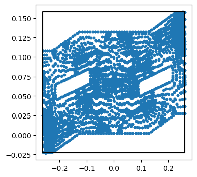
To make things more mathematical, I have a set of points in 2 dimensions (since I'm just looking for a top-down view), and I want to find a closed curve that contains all the points, but has the minimum area. As a zeroth-order approximation, we could just use a box with the minimum/maximum coordinates of all the points as the corners. That doesn't work very well for the set of points I was dealing with though:

Since this stage of the pendulum is tilted in these coordinates, we end up including a lot of empty space. We could do a little better if we rotated our box, but we're still not going to do great with right angles.

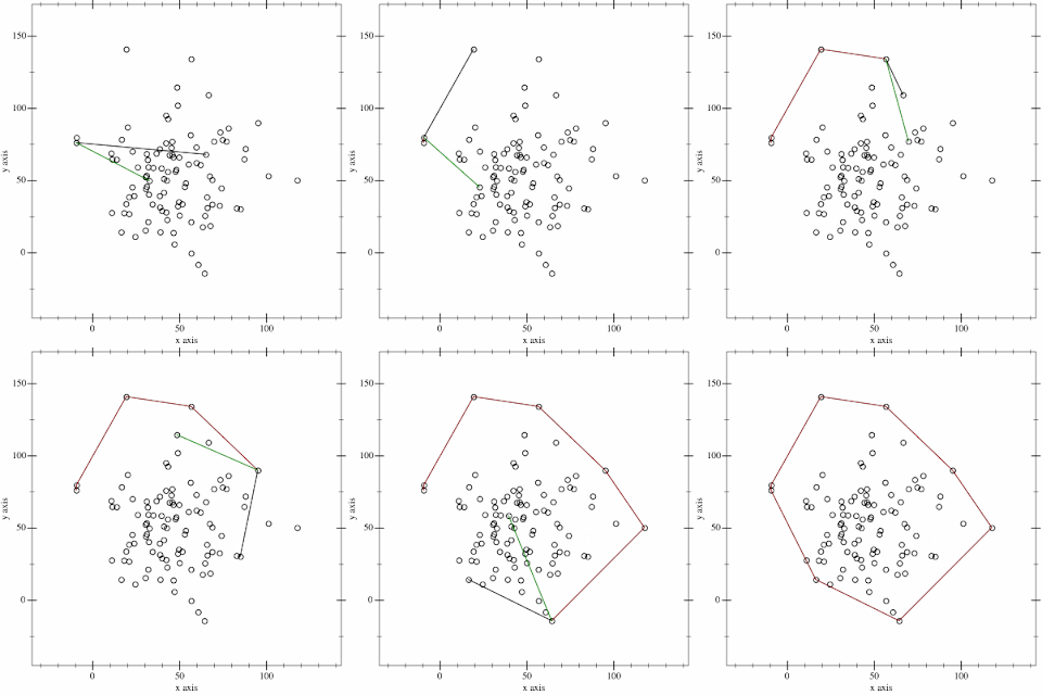
Another option is to try to find a convex hull. To get an idea what this looks like, you can imagine stretching a rubber band around the points. One method for finding the path is called the gift-wrapping algorithm, since it touches only the outer-most points, like wrapping a present. The algorithm builds up the path by looking for the largest angle to the next point. Wikipedia has a nice animation of this:

Wikipedia

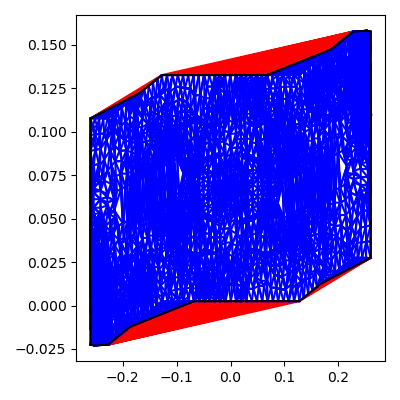
Unfortunately, this only works for convex curves, meaning the shape can't have dents, like our point set does. That brings us to the idea of alpha shapes. These start by dividing the shape into a set of triangles. Each triangle can be assigned a radius based on the size of the circle that would be needed to surround them. We throw out any triangles with radius larger than a given value, then find all the edges that belong to only one triangle – This is the border of our shape. Below are two examples of this for different alpha values, which correspond to the inverse of the radius limit. The red triangles are those that don't pass the limit.

α = 1

α = 2

Below is a comparison of the borders for a couple values of alpha. The first plot is the convex hull, using the Jarvis algorithm, another name for the gift-wrapping algorithm. The second plot, with α = 0, is the same, since that corresponds to an infinite radius, so all the red triangles from above get included.

Once the paper is more complete, I may discuss it here in full, but I'm glad I was able to learn about this technique, so my figures can be a bit more informative.

A Rainbow of Random

Last week I was talking to Steve and Nate (my father and brother), and they mentioned using white noise generators to help with sleeping. That made me think of a meeting I was in earlier in the week where someone mentioned that LIGO and LISA typically have red noise contaminating the measurements. That made me wonder: What does red noise (or other colors of noise) sound like?

First off, we need to talk about what it means for noise to have a particular color. In the context of light, color tells use the frequency of light: red light has lower frequency than blue light, and white light is a mixture of all frequencies. We can apply the same principle to frequencies of sound: more low frequencies is redder, and more high frequencies is bluer. We figure out the "color" of a dataset by taking its Fourier transform, and looking at where the peak frequency lies. White noise has an equal amount of power in all frequencies.

That's the theory, but how do we go about generating different noise colors? White noise is easy: Given some sampling rate, we generate uniformly distributed random numbers. Because these numbers are uncorrelated, they don't favor any frequency, and give a flat spectrum. We can "redden" that noise by giving each sample some dependance on the previous. This page suggests mixing each sample with part of the previous:

where x is the series of samples, w a series of white samples, and r a tuning parameter between 0 and 1, with 0 giving white noise, and 1 giving constant values. For blue noise, we want to do the opposite: sequential values should be as different as possible. To do that we can follow the method here: For each blue point we want to generate, we get several white points and pick the one furthest from a previous sample.

We still haven't gotten to what these different noises sound like though. For that, we can use Javascript's AudioContext, and pipe these sequences of values through your speakers. Below, you'll find a slider to control the color of the noise – For red noise, it represents the r from above, and for blue noise it represents how many samples ago to avoid. That technique isn't quite right, so for values above zero (which is the white noise point) there isn't a continuous transition. In the window above the slider, you can see the Fourier transform of the sound, with the frequency going left to right. Maybe not the most soothing sounds, but I hope it can give you some insight into the sort of problems scientists have to deal with.

Da Breeze of Debris

I recently saw a blog post suggesting publicly available datasets good for testing analysis techniques. Paging through them, I found the US Government's data server included NASA resources, and a connection to my own research occurred to me: One of my colleagues at the University of Florida has been working on simulating the effect of micrometeorite impacts on the LISA spacecraft. At a recent meeting, he was discussing the direction the meteorites might hit the spacecraft – They're generally falling inward toward the Sun, while the satellites (and the Earth) are orbiting around the Sun:

According to this model, very few meteorites should hit from the side facing the Sun. Less obvious though is the other 3 sides: Do more hit the side opposite the Sun, or is there a greater effect from the orbit taking us into the meteorite's path?

NASA's datasets include a record of meteorite landings on Earth, spanning the last 2 centuries, but unfortunately only provides the year, which means we can't find the Earth's position in the orbit. I almost gave up, but then I found a list of Fireball and Bollide Reports, which gives the precise date. Unlike the previous table, these are objects that completely burned in the atmosphere. We can look at the locations where these events were reported, using one of the map projections I discussed a while ago:

These appear fairly evenly distributed, but this plot doesn't consider the location of the Sun. Using the Astropy package, we can find the location of the Sun for a given date, then find the angle from the Sun to Earth, to the direction of the report:

This would seem to suggest that the most common angle is 90°, which corresponds to the orbit taking us into the meteorite. However, there are some significant caveats to this conclusion: It may be that there's a bias in this data, since it's easier to see a streak across the sky, while a meteor coming head-on would just appear as a point. Then there are the limitations of my analysis: The table only give the date of the events, not a time, so I may be introducing bias by choosing midnight. I'll be curious to see what results my colleague turns up, and maybe I'll find more datasets in the list to play with in the future.

Banditopod

Recently as part of my research, I've been trying to measure a probability distribution – specifically, the chances that we've seen a certain signal in LISA. The trouble is, there are many random noise factors that go into the calculation of whether we see the signal or not, so it's not a straight equation I can plug things into. Instead we need to sample it many times to estimate the distribution, and this can be expensive. My colleague Henri suggested I could use a technique called Markov Chain Monte Carlo (MCMC). I thought to get a better feel for the method, I'd try out a simple example here.

There's a traditional problem in probability theory called the "two-armed bandit." Imagine a slot machine with two levers – You insert a coin and choose which lever to pull. Each arm has a certain probability of paying out, but the only way to find out is by playing, and looking at how often you win or lose. What then is the best strategy for choosing a lever? You may have gotten lucky your first few pulls of one lever and overestimated its chances of winning.

We can make this more like my research by extending to a multi-armed bandit – Each arm represents a set of parameters we're searching for, and we want to pick the arm with the biggest payout/best fit to the data. Still to be answered though is how we pick which arm to play: Imagine a set of players, who can choose an arm at each step based on the wins/loses they've seen. Each one is more likely to pick an arm with lots of wins, but might try another arm just in case. Now, if we look at the estimated probabilities for each arm as time goes on, we might think we'd get a good idea of the true values:

The blue line is the true probability for each arm, and the orange dots are the estimates based on the average number of wins. The dots are jumping around so much though that it's hard to see how well we're doing. Instead of animating in time, we can try looking at how frequently we play each arm:

Pretty quickly, each arm gets a consistent rate of pulls, but it looks like we're undersampling the highest-probability arms. I think this may be due to the top-probability arms having fairly similar values – As I pointed out above, we can't tell whether we have the best lever, or just a streak of luck, so we hedge our bets. A common technique with MCMC is run a "burn in" for a while to let the players move around the parameter space, then reset the probability estimates and continue running.

As a final view of the data, we look at how the players distribute themselves among the arms through time [NB: The x-values are off by 1 compared to the earlier plot due to the way I gave the distribution to the MCMC tool I used]:

It starts off fairly flat – the parameter exploration I was talking about – but after a certain point, the distribution establishes itself, and from there the shape simply scales upward. However, even if you could afford to play tens of thousands of times, I think you'll be hard-pressed to find a slot machine paying out as frequently as these!

In My Corner

For a while I've been interested in analyzing the game Jenga, since it's very physics-aligned in its design: Maintaining balance under changing forces. I couldn't get a handle on how to look at it though, until I connected it to a tool that's used frequently in my research field: corner plots. Corner plots are a way to display correlations between different variables in a large data set. For gravitational waves, they're used to show how estimates of a source's parameters depend on each other, such as a black hole's mass and spin. I figured I could come up with some measurements of Jenga games, and look at how they relate to each other.

First, we need a way to collect some data. As a reminder, here's what a Jenga tower looks like:

Wikipedia

Each level has 3 blocks that alternate in direction. On a turn, we remove a block from anywhere below the top level, and then add it to the top. The tower will fall and end the game if the center of mass of a subset is over an empty space, and the side is not supported. I was able to make a simulation of this in Python, with the virtual player making a random move on each turn, so long as that move does not cause the tower to fall. Eventually, the player will run out of moves and the game will end, but we can look at what kinds of moves result in longer games. I struggled a bit to find a way to show an example tower being built, and settled on a side view with all the bricks facing out. Remember that the bricks actually alternate in direction, so a hole under a brick is not necessarily a problem:

Now to get our statistics, we want to run a large series of games, and get some measurements from each one. The parameters I chose were max height of the tower, number of turns taken, fraction of turns for which the center block of a level was removed, fraction of turns a block was placed on the center of the top, and the fraction of times a block was removed from the upper half of the tower. After running 500 simulated games, we can make a corner plot with the results (click to enlarge):

This shows us some interesting connections between our parameters. There is strong correlation between the maximum height and the number of turns – This makes sense, since each turn we put a brick on the top level. We can also see anti-correlation (negative slope) between removing the center brick and max turns/height. This is because once the center of a level is taken, we can't take either of the sides, so we run out of bricks faster. Our final two variables, adding to the center and removing from the upper half, don't seem to have much effect on the outcome, indicated by the circular distributions.

Now in reality, Jenga bricks are designed with some irregularities to make the balance a little more difficult to predict, so this is another case where knowing the physics might not help you win, but it was interesting way to explore a tool for visualizing data.

Sidebandits

This week was another LIGO-Virgo-KAGRA collaboration meeting, and since my work has focused on the detector itself, I tried to attend more of the sessions on instrumentation than I did in my data analysis days. One topic that stuck in my head was a technique for sensing the sizes of the various optical cavities used in the detectors, sidebands. By modulating the frequency of the main laser beam, we can effectively create frequencies on either side of the central one. This is the inverse of the effect I discussed way back in my PhD work.

"Modulation" simply means we're multiplying two sinusoids together, and we can apply a trigonometry identity to turn that into a sum:

This says that the frequency of the modulated signal is the sum and difference of the two frequencies that went into it. Often we add this modulated signal back to the carrier, z_1. Then we have three evenly spaced frequencies: f_1-f_2, f_1, and f_1+f_2, hence the name "sidebands". What's interesting is the variety of shapes you can get from this simple setup.

As a way to help me get my head around how everything interacts, I put together another doodad (two in a row!) which you can play with below. The top plot shows the timeseries of the signal, and the bottom plot shows the real part of the Fourier transform, a representation of the relative sizes frequency components. You can control whether we add the carrier to the modulated signal with the checkbox. I realize this is a somewhat obscure topic (and certainly not "everyday") but I hope it's fun to play with even if you're not as crazy as me!

Loops on the Ground

This week in one of my group meetings, a colleague presented her work on identifying and eliminating ground loops. I had never heard of the phenomenon, but it's an interesting pitfall in circuit design. When we talk about voltages, we always need some reference point – Voltage isn't an absolute value, but the difference between two points. When designing a circuit, it can be useful (and safer) to have a connection that can give or take current freely. This lets you get rid of excess positive or negative charges, like static electricity, that otherwise could damage components. This is why modern outlets have 3 connections: positive, negative, and ground.

When we connect devices together though, a problem can arise:

Here we have two components, both connected to AC outlets (+, –, GND). One of them sends a signal to the other. Since voltage is a difference, we need a second connection as reference, so we use the ground wire from the outlets. Now we have a loop of wire though – A loop is a type of antenna, which can pick up signals.

According to this article, the voltage produced by a small-loop antenna is

where N is the number of loops (1 in this case), A is the area, λ is the wavelength, E is the electric field strength, and θ is the angle between the loop and the signal. This article, about honeybee exposure to RF signals, gives the maximum electric field strength measured as 0.226 V/m. FM radio signals go up to about 200 MHz, or a wavelength of 1.5 m. If the area of the loop is 0.1 square meters, or about 32 cm per side, we can get as much as 95 mV of interference, easily enough to throw off a delicate measurement!

Marika's parents are visiting us right now, so I asked my engineer father-in-law Scott if he was familiar with ground loops. He related an interesting experience: He used to have a phone that he would plug into his car power, and an audio jack to play music through the speakers. The power and audio shared a ground connection, resulting in a loop that would add static noise on top of anything he played!

GRACE is Beauty in Motion

This week, I heard two talks on the Gravity Recovery and Climate Experiment (GRACE), an experiment being developed by some of my colleagues here in Florida. The goal of the experiment is to measure variations in the mass distribution of the Earth, using a pair of orbiting satellites:

JPL

As the satellites orbit, they pass over regions of greater and smaller mass, causing them to speed up or slow down. These variations will affect the leading spacecraft first, causing the separation between them to change. We can measure these changes with a laser interferometer, just like the ones used by LIGO and LISA. This results in a detailed map of how mass is distributed over the planet:

JPL

The heaviest points (in red) tend to be in mountain ranges, like the Alps and Andes.

You might be wondering (as I did) how this relates to climate. The key is that water is dense stuff, so when it moves around, it can significantly change the pull of gravity. As snow and ice melt, the water will flow to different places. The researchers have made their data available online, so I tried putting together some code to make summary plots.

The data I linked to above records the liquid water equivalent thickness, which is the depth of water over an area that would result in the measured mass per area. It covers 2002 to 2020, giving a planet-wide measurement every month. I plotted the data on a Mollweide projection and animated it in time:

I wasn't able to make it as clean as some of the diagrams the presenters showed, but you can see some seasonal variations, particularly in the Amazon region, and you can see things get significantly redder as time goes on. Looking at a single point in the middle of the North Atlantic shows an alarming trend:

As the glaciers and ice caps melt, that water flows into the oceans, raising the levels. On top of that, warm water expands, so any kind of heat added to the oceans will increase the depth. I hope we can use tools like GRACE to learn how best to reverse trends like this, and how to emphasize how necessary it is!

We Will Control the Vertical

[Title from The Outer Limits intro.]

Recently, my research has involved working with the control systems of the LISA spacecraft, which allow them to remain properly oriented. One of the main tools we use for this is a State Space Model. This type of structure models a physical system as a set of inputs, outputs, and states, which change in time. The system is defined by 4 matrices:

where u is a vector of inputs, y is a vector of outputs, and x is a vector of states. The dot indicates a time derivative, which tells us how the states change in time. Because this is a linear model, it will only work if we stay close to some equilibrium, but that's exactly what we hope to achieve. If we choose our inputs in relation to the outputs, we can try to stabilize the system.

I decided to play around with this model a bit by using the classic example of an inverted pendulum. This type of system may be familiar to you if you've ever tried to balance a pole on the palm of your hand. We want to keep the pole straight by moving its base. Gravity makes it tip in one direction or the other, and we react by moving our hand in the same direction. The trouble is how to avoid overshooting. For my model, I used a sliding cart in place of a hand. If we don't apply any external force to the cart, the rod will quickly fall over:

We want to apply a force to keep the cart underneath the pole, but I found that if I applied a force exactly opposite to the one making the pole tip, the pole would stay at a fixed angle while the cart zoomed off the screen. I played around a bit with different forces based on the pole's angle and speed, and found a configuration that looks pretty good:

It been interesting to learn some of the techniques that are more engineering-focused. I'm just glad I have more experienced people to help me out – I don't want to be responsible for another Mars Climate Orbiter!

A Breath of Fresh Vacuum

This past week was LISACon 8, a meeting of the LISA Consortium, similar to the LIGO meetings I've attended in the past. One of the presenters showed this daVinci-esque drawing of the LISA constellation:

ESA

A couple weeks ago, I talked about how I was working on a model of the rotation of the LISA satellites. Nominally, the satellites form an equilateral triangle, with 60° angles, but over the course of a year's orbit, those angles "breathe", getting wider and narrower as the spacecraft move along their orbits. That means that we need to change the angles the lasers point, so they can hit the distant sensors.

The laser beams are sent and received by Movable Optical Sub-Assemblies (MOSAs), the tubes in the picture above. We need to rotate those MOSAs to track the other satellites, but there's a problem: Angular momentum is conserved. Usually, we can count on the Earth to absorb extra angular momentum, but that's not possible in orbit. When we turn one of the MOSA, the spacecraft will turn under it. We can figure out how much using Newton's laws:

This says that the sum of the torques on each MOSA and the body of the spacecraft have to cancel out – "Every action has an equal and opposite reaction." We can use another of Newton's laws to express those torques in terms of the angular acceleration:

Here, the Is are the rotational inertia of the MOSAs and the spacecraft. The accelerations are measured in the inertial frame where all three bodies are rotating, but the MOSAs move within a range on the spacecraft, so we really want relative accelerations. We can get this by regrouping things:

We can make a bare-bones model by imagining two rods rotating in a solid disk to get I_M and I_S, then integrate to get the angles:

where m_S and m_M are the masses of the spacecraft and each MOSA, and φ1 and 2 are the angles of the MOSA relative to the spacecraft.

Eule Slick

A couple months ago, I talked about the LIGO work I'm doing here in Florida, but I'm also working on the LISA project, a gravitational wave detector in space. The detector consists of 3 spacecraft that orbit the Sun trailing slightly behind the Earth:

Wikipedia

Recently I've been developing a simulation of the LISA spacecraft, specifically their orientation to face each other. This gets into a part of Physics that I don't have a lot of experience with: rigid-body dynamics.

Most of the time, physicist can get away with considering things to be points or spheres, but things get more complicated with asymmetrical objects. Suppose we have a box that we want to rotate around two axes, x and y. Depending on which we do first, we get different results:

To get around this ambiguity, the mathematician Leonhard Euler (pronounced "oiler") realized you can specify the orientation of a 3D object by defining 3 rotations from a principle set of axes:

Wikipedia

I won't get into the details of how the angles are defined, but the result explains some really interesting effects. Here's a video recorded by a NASA astronaut aboard the space station of a "T-handle" spinning:

That strange tumbling behavior is explained by Euler's rotation equations:

where ω is the angular velocity, and τ is the torque applied. The I is the moment of inertia tensor, which requires some explanation: Simply put, it's the rotational equivalent of mass, which quantifies how a torque relates to an angular acceleration. What complicates things is that I depends on your choice of axes. It's a simple diagonal matrix in the frame where the T-handle is fixed, but that frame rotates. The fact we're working in a rotating frame results in the second term in the equation above.

Here's where the Euler angles come in: The differential equation above tells us how the angular velocity is changing, but we're interested in how the orientation of the handle changes. We need to relate the angular velocity to the change in the Euler angles, and include those in our integration. Putting everything together, we can simulate how the handle reacts to an initial rotation.

First with the spin perfectly aligned, nothing too interesting happens:

If we introduce just a 2% offset in the angle though...

we see precisely the sort of flip from the video! I've said it before here, but this is why I love Physics: With just a few relatively simple equations, you can explain even the weirder parts of reality.

Dentist Time

[Title from my grandfather's favorite joke: When is the best time to go to the dentist? 2:30! (Tooth-hurty)]

Earlier I said I would describe what I'm doing here in Florida, and this week I'm going to talk about my work on LIGO. I'm part of the engineering department here, so rather than the data analysis that I usually do, I'm more involved in the mechanics of the detectors. I described in my first post on LIGO how gravitational waves stretch and squeeze space. That stretching is a proportional factor, so the longer the distance, the greater the change. The scaling factor is so small though that to have any hope of picking it up, we need an enormous distance. The detectors are 2.5 miles long, but on top of that, we use resonant cavities that bounce the laser beam back and forth many times:

The laser goes through two partially-reflective mirrors that concentrate the light in a small area. The mirrors have to be precisely aligned to make the light add, instead of cancel out:

The laser we use in LIGO has a wavelength of 1064 nm, which means the difference between making the peaks add or cancel is only 0.000000266 meters!

This past week I was attending some (virtual) workshops on a tool we use to simulate cavities called Finesse. Adapting some of the code my colleague Luis Ortega wrote, I made a plot of the laser power that builds up in the cavity if we send a 1 Watt laser in, and have 85% reflective mirrors on either end:

One quality of a resonant cavity is how quickly the power falls off when the length is changed. Here you can see that if we have things just right, we can increase the power by 6.5x, but any error, and the output quickly drops to near zero.

The part that I'm working on is making simulations of the suspensions that help prevent the mirrors from moving out of alignment. Maybe in a future post I can discuss that, but I wanted to start with the basics, since I haven't been thinking about this stuff for as long as my coworkers.

Filling in the Holes

Following up on some previous posts about gravitational wave detections, this week I have some questions from Papou:

How many current black hole collisions are we aware?
Last year, the LIGO/Virgo Collaboration released the first Gravitational-Wave Transient Catalog, covering all the detections from the first and second observing runs. That includes 10 binary black hole (BBH) events, and 1 binary neutron star (BNS) merger. The third observing run is split in two pieces. Results from the first half, O3a, are available on GraceDb, and include 37 BBHs, 6 BNSs, 5 neutron star black hole (NSBH) mergers, and 4 events that fall in the "mass gap".

The mass gap represents a range of masses where we have never seen a black hole or neutron star. This image shows a summary of the compact objects observed by LIGO and electromagnetic astronomers as of the end of O2:

via Northwestern

The empty space between 2 and 5 solar masses is the mass gap. It is unknown what kind of bodies were involved in those mass gap collisions.

What happens to "Matter and Antimatter" when two black holes collide?
Black holes are made of matter. When matter and antimatter combine they make energy, but as with most physical processes, this is reversible: energy can create matter/antimatter pairs. Since the universe contains residual heat energy from the Big Bang, these pairs are constantly forming and annihilating back into energy in space. If one of these pairs forms near a black hole though, the antiparticle can fall into it, while the matter particle escapes. This process is called Hawking radiation, and can lead to a black hole losing mass.

Are photons escaping due to the collision energy?
In the case of black holes, no. Light can't escape a black hole's event horizon, and when two collide, their horizons merge. Neutron star collisions, however, can release photons in the form of a gamma-ray burst (GRB). In an earlier post, I mentioned LIGO's detection of GW170817, which showed a correlation between a binary neutron star merger, and a GRB.

Are the combining gravities simply arithmetic additions or does the total gravity grow in multiples?
Neither! Mass and energy are connected through E = mc^2, so when energy is released in the form of gravitational waves, part of that comes from the masses of the black holes. Despite the extreme sensitivity needed to detect gravitational waves, they carry an enormous amount of energy. The first detection, GW150914, lost about 3 suns worth of mass-energy. I tried to find a way to put that number in perspective, like "X billion nuclear bombs", but it's so huge that it dwarfs even a measure like that. Spacetime is exceptionally stiff stuff, and wrinkling it even a little needs an amount of energy that we don't normally encounter.

Thanks for more great questions, Papou!

A Singular Family

This week, I got some great questions from my nephew Ezra, along with his parents Nate and Carrie. I gave them some quick answers off the top of my head, but I thought they deserved a more in-depth treatment as well.

Ezra: What does a gravity wave feel like [to a person]?
As a reminder, gravitational waves warp space as they pass. If a wave passed through the center of a hula-hoop, it might look like this:

Each image is a point in time. Adapted from my thesis.

Gravitational waves are incredibly weak, which is why we need 2.5 miles of detector to pick them up. They’re a squeezing and stretching of space, so if you could feel them, they’d be a combination of a hug (awww) and a medieval rack (ahhh!). Some of the early detectors were big pieces of tuned metal that scientists hoped would ring like a xylophone if the correct frequency passed by. Those were never sensitive enough though.

Nate: But aren't they weak because they're distant? What if you were closer to a pair of black holes approaching collision? Could you be close enough to feel the waves but far enough to not be inside?

Good point! We can take the first LIGO detection, GW150914, as an example. According to that paper, the distance was about 410 megaparsecs, and the peak strain was 10^-21. Strain is the fraction by which the wave changes distances, so a meter stick would be stretched and squeezed by 1/1000000000000000000000 meter! That's pretty tiny, but strain drops off as 1/distance, so we can get a bigger effect closer to the collision. We probably don't want to be inside the event horizon of the final black hole, which has a radius of

Plugging in the 62 solar masses from the paper, we get 183 km. Supposing a 6 ft person observed the collision from 200 km away then, their height would change by a little over 4.5 inches!

Carrie: Is a black hole a hole in space-time or a depression?

It's both! -ish. This is a difficult question to answer, since the whole point of a black hole is that we don't know what's going on inside it. The trouble is that when a star collapses into a black hole, it creates a singularity – a point of infinite density. That creates a lot of problems for General Relativity, since things falling into the singularity could wind up going faster than light, and other bad things that happen when you have an infinite quantity. Instead, we put an event horizon around the singularity at the point where light can no longer escape from it, which is usually where bad stuff starts. Wikipedia has some nice representations of a singularity with and without an event horizon (bad stuff not included):

Black hole, via Wikimedia Commons

Naked singularity, via Wikimedia Commons

Thanks for some great questions!