The Summer of Heat & the Winter of Desiccation

Thanksgiving put baking on my mind, and I started thinking about a post I wrote several years ago about baking a cake in different sized pans. I had been concerned in that post that I didn't take into account the evaporation of water from the cake, which would change the way it heated. This week though, I thought of a way to account for that, and decided to follow up on my previous post (and continue the French Revolution theme).

To recap, my mother Sally was baking a cake, but her pan was smaller than the recipe called for. That meant the cake would be thicker, and she wondered how that would change the cooking time. The key to figuring out how temperature changes spread through an object is the heat equation:

This says that the change in temperature at a point is proportional to the variation in temperature at the surrounding points. I mentioned last time that it was the proportionality constant, α, that depended on the moisture content of the cake batter. I realized that we could account for a changing amount of water by varying α according to

where m is the mass of water and of other ingredients in the cake, and α the individual diffusivities. I was surprised to find that a group of food engineers (!) had actually measured the thermal diffusivity of flour. Taking a sheet cake recipe as an example, we can approximate the amount of liquid (~water) and the amount of flour to get the effective α.

It still remains to determine how the amount of water changes over time. I looked into a couple ways to tackle this, and I'm not sure how accurate my technique is, but it made the most sense to me: The particles of a substance at a certain temperature have a statistical distribution of energies. For ideal gases, there's the Maxwell-Boltzmann distribution, and even though that's not a great model for liquid water we'll go for it. It takes a certain amount of energy for water to evaporate, called the heat of vaporization. If we assume that all the molecules with this much energy do leave the solution, we can keep track of the current number of water molecules still in the cake. Taking out those high-energy particles will also cool the cake, so we can figure out the temperature change with the heat capacity.

I updated the previous code to include these new modifications. Once again, we start off by measuring the temperature after a given amount of time using the wider pan:

In contrast to the previous results, the center temperature goes well above water's boiling point! We can also look at how the amount of water changes over time:

I was surprised to see that the center of the cake experiences almost no loss in water. Even the edges don't lose much – The color scale varies from 50 to 60%. To check what effect the loss of water has, I reran the test with the same α calculated above, but left the amount of water constant. The results are almost identical:

As in the previous post, we can use that central temperature as a target for the narrower pan, and find the cook time:

As before, we get about 70 minutes, suggesting the water content is not as significant as I imagined. A big part of physics is figuring out what you can approximate, and what you can't – which results are "good enough". It seems cakes can be quite forgiving when it comes to baking precision!

Sowing Division

We have several recipes that make 6 servings, and I always have a hard time dividing them equally. It seems I have an easier time splitting things in 2 rather than 3 or other divisions – I assumed this was a human tendency, but I can't turn up anything from searches. While cutting up a casserole one evening, I started thinking about how after cutting 1/3, the next cut would be half of 2/3. Instead of making that cut, I could mark the half and then flip the relation: I have a new 1/3, and I can split the remaining 2/3 in half.

We can put this idea in more mathematical terms: I want to place points a and b on a line of length 1 so that a = 1/3 and b = 2/3, but I can only put them at halfway points. If we start with a0, then b0 goes at (1 + a0)/2. If we keep going back and forth, then

Writing out the first few terms of the sequence for a lets us identify it:

The term in the parentheses is a geometric series, which can be replaced with a simple form. After some rearranging, we get

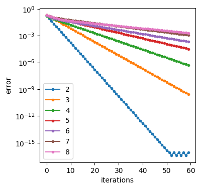
I realized this technique could be applied to any number of cuts by adjusting each to the center of the two neighboring cuts. Finding an expression for the general case is "left as an exercise to the reader" (textbook cop-out) – I just tossed the algorithm into Python. The main thing I was interested in was how long it takes to get an accurate estimate of the divisions, so I plotted the RMS error at each step:

Each line represents a different number of cuts. Notice that the y scale is logarithmic, meaning these straight lines actually represent exponential decreases. The line for 2 cuts into 3 pieces drops so quickly, it appears to run into some precision error. As the number of cuts increases though, the error is much more difficult to reduce. To get a more concrete handle on this plot, I also made an animation of the cuts as we make iterations:

For the first step, the divisions are evenly distributed at the two endpoints, which is really a worst case scenario. However, we can see how quickly the 2 cuts on the first line settle in place. Moving up the plot, each line takes a little longer to stabilize.

I'm not sure my serving-precision needs are high enough to require actually using this technique, but it was interesting to think through!

Eule Slick

A couple months ago, I talked about the LIGO work I'm doing here in Florida, but I'm also working on the LISA project, a gravitational wave detector in space. The detector consists of 3 spacecraft that orbit the Sun trailing slightly behind the Earth:

Wikipedia

Recently I've been developing a simulation of the LISA spacecraft, specifically their orientation to face each other. This gets into a part of Physics that I don't have a lot of experience with: rigid-body dynamics.

Most of the time, physicist can get away with considering things to be points or spheres, but things get more complicated with asymmetrical objects. Suppose we have a box that we want to rotate around two axes, x and y. Depending on which we do first, we get different results:

To get around this ambiguity, the mathematician Leonhard Euler (pronounced "oiler") realized you can specify the orientation of a 3D object by defining 3 rotations from a principle set of axes:

Wikipedia

I won't get into the details of how the angles are defined, but the result explains some really interesting effects. Here's a video recorded by a NASA astronaut aboard the space station of a "T-handle" spinning:

That strange tumbling behavior is explained by Euler's rotation equations:

where ω is the angular velocity, and τ is the torque applied. The I is the moment of inertia tensor, which requires some explanation: Simply put, it's the rotational equivalent of mass, which quantifies how a torque relates to an angular acceleration. What complicates things is that I depends on your choice of axes. It's a simple diagonal matrix in the frame where the T-handle is fixed, but that frame rotates. The fact we're working in a rotating frame results in the second term in the equation above.

Here's where the Euler angles come in: The differential equation above tells us how the angular velocity is changing, but we're interested in how the orientation of the handle changes. We need to relate the angular velocity to the change in the Euler angles, and include those in our integration. Putting everything together, we can simulate how the handle reacts to an initial rotation.

First with the spin perfectly aligned, nothing too interesting happens:

If we introduce just a 2% offset in the angle though...

we see precisely the sort of flip from the video! I've said it before here, but this is why I love Physics: With just a few relatively simple equations, you can explain even the weirder parts of reality.

Learn All That is Learnable

[Title from Star Trek: The Motion Picture, V'GER's mission.]

Earlier this week, the Voyager 2 spacecraft broke an 8-month silence to check in with NASA researchers. This is one of the most distant space probes from Earth, currently about 11.6 billion miles away. It was originally launched in 1977, with the primary goal of observing Neptune and Uranus. To get to those planets in 1989, it was given enough velocity to leave the solar system entirely, which it did 2 years ago. The antennas that communicate with Voyager, called the NASA Deep Space Network, were under maintenance for the past 8 months, preventing contact.

After seeing the news article about the renewed contact, I started reading more about the probes, and how they achieved their Sun-escaping speed. They key lies in the idea of a gravity assist, where by flying by a planet in the right way, an object can get a boost of speed:

Wikipedia
   Voyager 2 ·   Earth ·   Jupiter ·   Saturn ·   Uranus ·   Neptune ·   Sun

The principle at work in a gravity assist is actually something usually taught in intro Physics: an elastic collision. This is when two (or more) objects interact in a way that conserves both energy and momentum. An everyday example is a rubber ball that bounces to its original height when dropped. The energy and momentum of an object are given by

where m is the mass and v is the velocity. Conserving these quantities means that before and after the collision, the sums of each one for all the objects involved stays the same. To simplify things, we can consider the case in one dimension: Initially the probe and planet are moving toward each other, the probe slingshots around the planet, and leaves in the opposite direction it came. Then we can use the elastic collision equations to get

where capital variables are for the planet, lowercase for the probe, and i and f for initial and final. Since planets are generally a lot bigger than space probes (though maybe not in the case of the source of this post's title), we can Taylor expand around m/M ≪ 1 to get

Jupiter's mean orbital velocity is about 13.1 km/s, or about 30,000 mph, and we could get double that! Unfortunately, the angles typically don't work out that way, as you can see in the animation above.

I feel that any discussion of the Voyager Spacecraft has to include the hope that went into creating them, and to that end, I want to end this post with a picture of one of the Golden Disks. Each of the spacecraft was loaded with a message to the stars about Earth and its people. We looked for a way to represent ourselves to the cosmos, and found what was best in us.

Pitching Forward

In their house in Ashfield, my parents have a 500-foot well that delivers their water. Growing up drinking that delicious water has spoiled me for most municipal water supplies, including the one here in Gainesville. To appease my picky palate, we got a filter:

The tap water goes in the reservoir at the top, then drains down through the filter to the bottom. It's possible to pour filtered water while some is still in the top area, and it made me wonder how the pitcher's center of mass changes as it tips forward, and as the water drains through.

The first problem is to find the shape of the water when the pitcher is tipped at an angle. The surface of the water will stay horizontal, so if we imagine tipping to an angle θ, we can instead imagine the pitcher flat, with the water at the angle:

Looking from the top, the pitcher is approximately an ellipse:

We're looking for the center of mass of the water, which is given by

where M is the total mass, and ρ is the mass density. This is essentially the weighted average of the position of each bit of water. Since water has uniform density, we can replace ρ and M with the total volume. Figuring out the limits of integration is a bit tricky: We can imagine moving in the x direction in the diagram above (left to right) adding up squares of water. The widths will be

and the heights will be

This makes the integral pretty ugly, so I threw it into Mathematica for an answer:

That's just for one of the water reservoirs; to get the CM for both, we weight the positions by the amount of mass in each. Since we're interested in tipping the pitcher forward, we can measure the angle of the CM from the front edge:

Remember though that we're also tipping forward by θ, so for the tipping point, we're looking for θ + φ > 90°. I put together some Python code to find the CoM angle for various tipping angles and points in the filtering process:

I find it really interesting that under this model, the 90° tipping point stays nearly constant. However, this fails to account for when there is not enough water to cover the bottom of either reservoir. From experience, I certainly don't feel the pitcher falling forward as early as 9 or 10 degrees. I tried to account for that in the integral, but the lack of symmetry makes it too difficult for Mathematica to handle. Even with that missing piece, an interesting system to analyze!