Pneumatic Drop

Now that we're in Florida, and no longer sheltering from COVID, I've actually been working on campus. My department is in the (slow) process of moving to a new building, so I've been temporarily put in one of the large offices shared by grad students, and I've noticed an interesting quirk of my chair: After I get up, now and then it will sink to its lowest height, so I need to raise it again when I sit down. I was curious what was going on, and decided to look into how the lift mechanism works (or doesn't).

Most office chairs use a pneumatic cylinder to set and maintain a given height. They consist of a tube that can let air in or out when you open a valve, a piston connected to the chair, and a spring linking the tube to the piston:

We've defined a few variables here: L is the uncompressed length of the spring, i.e. the maximum height of the seat, hset is the height the chair is set to when the valve is closed, and h is the rest height. Using these, we can write the 3 forces acting on the seat:

where patm is the atmospheric pressure, A is the cross-section of the cylinder, k is the spring constant, m is the mass of the person on the chair, and g is the acceleration from gravity. If we set F = 0, we can get the rest state of the chair, and try a few values for the various quantities:

Here we've solved the above equation for h, and then plugged in a bunch of values for m and hset. I chose L to be 15 cm, A to be for a diameter of 5 cm, and set k so that 40 kg can compress the spring by L. The black lines show some constant values for the rest height, which gradually change slope depending on the set height. I decided to replot these points to better show the relationship between the set height and the rest height:

The dashed line shows points where the chair does not move from its set height – I was surprised to see so many points above the line, meaning the chair rises from its set point, but I'm thinking that's due to the spring strength I used, which may be way off.

As interesting as this was to work though, it doesn't bring me any closer to explaining why my chair drops while I'm not sitting on it, rather than rises. Time to write a grant proposal for "Pneumatic Posterior Support System Instabilities: Sources & Solutions"!

Stopping Traffic

Since coming back to Florida and commuting every day, we've noticed that the traffic lights stay on a particular direction for a long time before switching. This is especially annoying as a pedestrian (who dislikes jaywalking), since it means the walk from the parking lot to my office can vary a lot depending on what lights I hit. I was curious whether I could design a simulation to test the effect of the light duration on the time cars spend waiting.

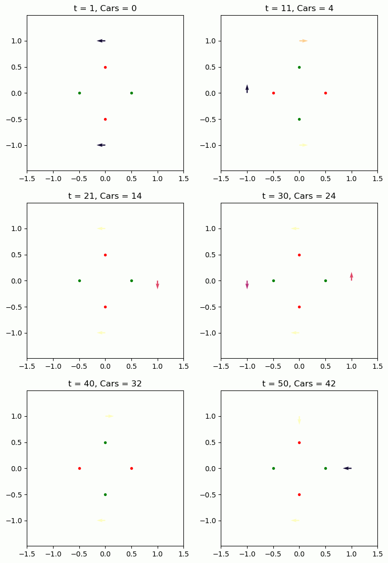
The setup is a 4-way intersection with lights that swap red/green with separate green durations for North/South and East/West. Each road has a rate cars arrive, and each car randomly chooses to go left, right, or straight. As cars pass through the intersection, we can keep track of how long they had to wait since arriving. Below is an example simulation – The arrows are the lead cars on each road, pointing in their planned direction and colored to indicate how long they've been waiting.

We've got a lot of variables going on here, so it took me a while to figure out how to assess the results. It would take too long to try every combination, so I just sampled from a reasonable-sounding range. I considered using a corner plot to see the effects of the inputs, but the sampling was too sparse to see a trend. One way to reduce the number of parameters is to consider where each car is coming from, and use the traffic rate and light duration from that side. Then I thought about the units: the traffic rate measures cars/time, and the light duration is a time, so multiplying them gives an average number of cars during a green light. Plotting this with the waiting time shows a clear trend:

I separated out the different turning directions, expecting that left turns would need to wait longer, but that doesn't seem to be the case. This shows that to minimize the waiting time, we need to keep the rate*duration small, i.e. for busy roads the lights should change rapidly, which is not what I expected.

This also implies that the Florida lights are expecting a low rate of traffic – Not our experience the past few weeks coming home during rush hour and hitting gridlock! Of course, this model may be inaccurate, and I should stick to gravitational waves, rather than civil engineering.

Dribble Cup

Earlier this week, I took my water bottle out of the fridge and, without thinking, put it near the small heater we had running. In seconds it was spewing water all over the table!

I figured the heat made the air at the top expand, pushing the water out through the straw, but what I was really curious about was: Does the amount of air the bottle starts with change how much water is forced out?

Air follows the Ideal Gas Law, which is given by

where P is pressure, V volume, N number of molecules, k Boltzmann's constant, and T temperature in Kelvin. That last bit is important: We usually measure temperature in degrees Fahrenheit or Celsius, which can be negative. Kelvin on the other hand is only ever positive: 0 K corresponds to absolute zero. We can convert from Fahrenheit with

In our situation, the temperature rises, which increases the pressure the air applies to the surface of the water. This pushes water out, increasing the air's volume, and bringing the pressure down. At equilibrium then, we can set the initial and final pressures equal. Similarly, the number of molecules won't change, since no air is entering or exiting. Using that, we can write the ideal gas law for the initial and final states, then set them equal:

What we're really interested in though is the change in volume, since that tells how much of a mess we're making:

We can plot this for a couple different initial volumes over the temperature range from refrigerator to heater-adjacent:

The green line is half full for my water bottle, and will spit out a couple tablespoons worth! As I write this, Marika is using the Instant Pot for some dinner prep – I'm surrounded by pressure vessels ready to blow!

Vanishing Trick

Back in March, I was at the LIGO/Virgo/KAGRA meeting, and during breakfast one morning, a fellow researcher posed an interesting question: Suppose a cluster of stars are all moving in the same direction. What can we learn from their vanishing point?

The concept of a vanishing point is often used in art: When parallel lines recede into the distance, they appear to converge at a point on the horizon. It seems logical then that our parallel stars will also converge to a point in the sky, which could tell us about how they're arranged in space. First though, we need to be able to generate a set of parallel lines in 3 dimensions. In 2D, this is fairly simple: Any lines with the same slope but different intercepts will be parallel. I found a page giving a simple way to express 3D parallel lines using a "double-equals" form:

The intercepts for each line are different, but the slopes associated with each dimension must be proportional between the lines.

This format is a bit difficult to imagine plotting, but we can fix that by setting the three terms equal to a parameter t, and then solving:

Once we have the paths in x, y, z, we can transform them into the right ascension and declination angles used by astronomers:

We have all the machinery in place now, so let's try it on a trio of lines. First, we can look at them in 3D, to check that we got parallel lines as expected:

Looks good! Now we'll run it through the projection...

Uh oh, the three lines don't share the same vanishing point! For a while I was sure I had made a mistake somewhere, but I think this can be explained by the fact that we're projecting onto a sphere, not a plane, as is usually done. I made a feeble effort at proving this to myself, but we're still running ourselves ragged getting things set up in our new home in Florida (hence the long silence here)!

Losing My Marbles

Next week, Marika and I will be flying to Massachusetts to visit my parents, and receive the generous gift of their camper van! Our trip happens to overlap which a favorite event on my childhood, the Ashfield Fall Festival. It includes local art, music, and cooking, but I was always more interested in the games. There was the usual tipping ladder, but my game of choice was the marble rolls. These were made from boards tipped at an angle with a grid of nails pounded into them. Rubber bands were stretched between nails in a pattern so that a marble dropped from the top would bounce off the nails and bands until it landed in one of the slots at the bottom. Different slots were worth different points that would determine your prize. I've now been studying physics for half my life, so I thought I could look at the game not as lottery, but as a deterministic physical system, and maybe win myself some grand-prize trinkets on this trip!

As the marble rolls down, it hits nails and bands that change its direction. Physicists typically look at collisions from two extremes: elastic and inelastic collisions. In both cases, momentum is conserved. For elastic collisions, energy is also conserved, but inelastic collisions in which the objects "hit and stick," or finish with the same velocity, lose the most energy possible while maintaining momentum conservation. For collisions between our marble and the nails/bands, the velocity we care about is only in the direction connecting the two objects: both collisions will stop the marble from going through it, but keep the component of velocity perpendicular the same. For nails we'll use inelastic collisions, which simply stop any motion through the nail, and for rubber bands we'll use elastic collisions, which reverse the direction.

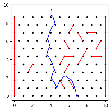
I wrote some Python code to simulate this, randomly choosing pairs of adjacent nails to stretch bands between. Checking when the marble hits a nail is pretty simple, since we can just get the distance between the points and see if it's within the radius of the marble. The bands are a bit more involved: we have a line segment between two points, and need to know the distance to a third point. The closest point on the line segment will be on the perpendicular that passes through the marble's center (proof left as an exercise for the reader, heh). I ran into a couple edge effects in the simulation, where the marble would get sort of "hooked" on one of the nails, but overall I'm pleased with the results:

Now that we have this basic framework, we can generate a board, then map out the landing positions for all the different starting points. I decided to make a sort of flip-book with different numbers of bands, randomly chosen. The starting positions are shown by different colored lines, and the bottom of the plot shows a histogram of where the marbles land.

I couldn't figure out a good way to get statistical measures, but it's interesting to see the gaps just below bands where no marbles pass through, and to see cases where a marble starting on one side of the board crosses to the other side. The 0-band case has a nice symmetry to it, and some of the middle ones look a bit like Jackson Pollock paintings, but the important part is, with this on my side, that plastic lobster harmonica is mine!

On My Soapbox

I've been applying to a bunch of faculty positions recently, and one requested a recorded teaching sample. I made this, giving an introduction to special relativity. Questions & feedback are welcome!

Mixed Signals

Recently for my research I've been working with digital signal filters, which are a way to change the frequencies that appear in a signal. Specifically, I've been using a Kaiser bandpass filter, which removes frequencies outside a given range. You might imagine that if we want a specific range of frequencies, we could just use a Fourier transform to set those points to zero. There's a problem with that though: In order for the transform to be precise, we need infinitely long data, so we can capture all frequencies. Since ours is finite, we will get spectral leakage, where the timespan of our data will introduce its own frequency to the spectrum. We can mitigate this by applying a window to the data, which tapers at the ends.

These filters are often displayed through their finite impulse response (FIR), which shows what the filter does to a single spike of signal. Below are responses for a square window, which corresponds to the sharp clipping I described above, and an example Kaiser window:

Notice that the square window has much more wiggling on the sides, while the Kaiser window damps out quickly. On the other hand, we do lose a little bit of power in the main lobe of the Kaiser – There are always tradeoffs in these situations.

Once we have the FIR for a filter, we can apply it to a signal with an operation called convolution:

You can picture this as sliding the filter across the signal and taking the sum of the product at each point – The Wikipedia article I linked has some nice animations. What I wanted to know was, how do the different settings for the Kaiser filter affect the result for the signals I'm working on? Below, you'll find a plot of a square pulse before and after filtering. The controls are the attenuation outside the band of desired frequencies, the width of desired frequencies, and the cutoff, which is related to how long the transition from the passed to the attenuated frequencies lasts.

Head's Up

Recently, I saw my father-in-law Scott pour a bottle of beer into a glass, and I was fascinated by the relationship between the rising beer at the bottom, and the foam moving on top. I was curious if I could model the dynamics involved, so I decided to check if anyone else has tackled the problem. I found an article from a brewer discussing some of the steps involved, and I decided to split the process into 4 parts:

1. For each bubble in the foam, apply forces from neighboring bubbles, and gravity pulling down.
2. Drain liquid from higher to lower bubbles, based on the content of each. Bubbles at the bottom drain into the liquid beer.
3. If neighboring bubbles each have low liquid content, merge them into a single larger bubble.
4. Bubbles with low liquid and/or large size pop, adding their liquid to the beer at the bottom.

To represent these bubbles, we need to use sphere-packing to figure out how they fit in the glass. I've talked about the concept before, but since we're making a simulation this time, I found the package spack for Python. This handles keeping track of where the bubbles are, and can draw them for us. It also calculates the forces between the bubbles, based on their separation and radii.

To apply these forces, we need the mass of the bubbles – They're made of gas and liquid, but the liquid mass will far outweigh the gas. We're already keeping track of liquid content for the other steps, so we can use that for the mass and then displace each bubble based on the total force divided by its mass.

The spack package keeps track of which bubbles are adjacent – For each pair, we can drain liquid from the upper to the lower. The proportion I settled on was that at each step the lower bubble would get 51% of the total moisture, and the top one would be left with 49%. For bubbles with nothing below them, they drain the full amount to the liquid at the bottom. Similarly, we can use the adjacent list to pick bubbles to merge – Based on the article I linked above, I decided their circumferences would add, rather than areas. We select which bubbles merge based on their liquid content – Dryer bubbles merge more easily. Big, dry bubbles can also pop, giving up their liquid to the beer at the bottom.

We start off the simulation by filling the glass with a bunch of small bubbles, then let the rules outlined take over. I ended up using 1000 bubbles to start with, which takes a bit of time to get through, but I'm impressed with the results:

We can also measure some averages over the course of the simulation. First, we can simply count the number of bubbles:

The rate is fairly constant, despite the various dynamics going into determining the merging/popping. We can also look at the average size of bubbles:

I was a bit surprised by the sudden rise in the average size at the end, but I think it may be related to the merging of the bubbles: They get larger and fewer, resulting in a compounded effect on the average, and near the end, we have far fewer bubbles, making the average more sensitive to change. The average liquid content has a similar knee at the later times:

I have no idea how accurate this model is, but it does seem to follow the events outlined in the article: Bubbles merge, dry out, and pop, resulting in a shrinking head of foam, and growing reservoir of liquid at the bottom. Clearly I need to gather more data – Cheers!

Maximized Magnets

Recently another post from Hack-a-Day caught my eye, discussing a technique for stacking magnets to get a stronger field, called a Halbach Array. You might assume that if you have a bunch of small magnets, the best way to combine them would be stack them with all their poles pointing in the same direction, but it turns out you can get a stronger field by stacking them in an unintuitive pattern:

Wikipedia

The arrows point from south to north pole of each magnet. Using the (wonderfully named) Python package Magpylib we can look at the magnetic field produced by this combination:

The field strength is represented by a higher density of lines, but that's a little hard to read off this plot, so we can also plot the overall magnitude of the field on a line just above and just below the magnets:

Not only is the field stronger than a single magnet's, it's stronger on one side than the other! This gave me pause, since it sounded like a monopole magnet, which is forbidden by Maxwell's Equations, specifically Gauss's Law for Magnets:

This says that for any closed surface S, all the field lines going out of the surface need to be matched with lines coming in, so that the sum cancels. It seems like our setup could have more lines going out the bottom than coming in the top, but the key is that even though the magnitude of the field is stronger on one side of the array, it includes both north and south poles. You can see this in the field plot above: there are lines going in and out on both sides. We can double check by integrating around a box as S:

When the loop closes, we're back to zero, and no laws are violated!

That last section may have been a little technical, so I'd like to end on something (I find) beautiful. In the Wikipedia article for Halbach arrays, they mention a version using magnetic rods, which can be rotated to switch the field from one side to the other. I was curious how the field strength varied during this, so I made an animation with the output from Magpylib:

The dots mark the north pole of each rod. Each 90° rotation swaps the strong side, but I think the movement of the 3 low-field nodes is really cool. Thanks, Hack-a-Day, for introducing me to this nifty structure!

Nega Millions

The Mega Millions lottery has been in the news a bunch lately, due to the growing jackpot, and I wondered how big the jackpot would need to be for it to be worthwhile to play. Specifically, I was curious about the relationship between the jackpot and the number of players, and exactly how unlikely winning is.

In many articles I found, like the one above, I saw the probability quoted as 1 in about 300 million, but I wanted to go through it myself: As of 2017, the drawing involves 5 numbers chosen from a set of 70, and 1 chosen from a set of 25. The order doesn't matter, so we can write this as

where the exclamation mark is the factorial operator, defined as n! = n*(n-1)*(n-2)*...*2*1. If you do this calculation, you'll find the number given elsewhere – Initially, I thought the order did matter, in which case the 5! would be left out, and there would be significantly more possibilities.

The total jackpot starts at $20 million, and then grows based on the number of tickets sold. We can look at how the jackpot has changed over the past year:

Each time the jackpot is won, it drops back to the baseline $20 million. The slope of the climb depends on the number of players – Note that as the jackpot increases, the slope of the curve also increases. When discussing outcomes with different probabilities, mathematicians often use the expectation value, a weighted average using the probabilities as weights. Since multiple winners split the jackpot, we can write the expectation value for the payout as

The chance of winning is 1/C; the chance of not winning then is (1 - 1/C). If k people out of N players win, we can raise the respective probabilities to the power of k and N-k to compound them. Now we can look at the relationship between the jackpot, number of players, and expected payout:

A couple interesting features of this plot: $500 million appears to be a threshold for a lot of people – The slope of the points increases here, suggesting people outside the set of regular players have joined in. Due to the low chances of winning, the expected value only barely passes $4, although that does exceed the purchase price of $2, so buying a ticket is "worth it" (if you ignore the time cost of buying the ticket and checking the numbers). The low win probability also means that the multiple winner aspect is pretty insignificant. For the numbers I used here, it didn't seem to change anything from the base winning number.

Th other thing I was interested in was how many drawings passed between wins. We can split the data up based on when the jackpot resets to $20 million, and then plot the curves on top of each other:

There are several that last only a couple days, but I was really surprised that the longer-lasting ones have almost identical changes in the number of players over time. That suggests the threshold behavior I mentioned earlier also applies on a smaller scale: As the jackpot grows, there's a continuous increase in the number of people willing to take the chance.

Going into this, I was already confident that playing the lottery was a terrible idea, but to me the expected value really drove that idea home: Even a record-setting jackpot will only barely push you over the break-even point.

Birefringe Benefits

This week, I set a plastic container on our kitchen counter in the sun, and noticed an interesting effect:

The reflection of the sunlight off the counter gave a rainbow pattern. I recalled seeing a similar effect in demonstrations of polarized light. The stresses frozen into plastic cause a change in the light's polarization, which you can observe by putting it between two polarizing filters:

Wikipedia

I've mentioned polarizing filters before, in the context of reflection, but as I thought about this situation more, a problem occurred to me: The plastic is birefringent, which means it rotates the polarization of light passing through it, but the light from the sun is unpolarized, so rotating it should have no effect. The light only gets polarized afterward when it reflects off the countertop. To understand why, I have to get into the weeds a bit, so I suggest reading that earlier post I linked to before continuing.

Oscillibations

A common question that arises for over-caffeinated physicists is, why does carrying a mug of coffee make it slosh over the rim? Ever since Marika got us our Apple Watches, I've been wanting to use the accelerometers in the watch, which allow it to measure your arm's orientation and motion, to record how my hand moves when walking with a mug. Sadly, I couldn't find an app that would allow me to download the data... until now! I recently decided to have another look, and found HemiPhysioData, designed to help people recovering from injuries track their progress regaining movement.

Accelerometers are a type of sensor that measure acceleration in a particular direction. A simple example is a weight on a scale: This measures a force, which is a mass multiplied by an acceleration. Typically these are used with just the acceleration due to gravity, but if you lift or lower a scale suddenly, you can increase or decrease the acceleration it reads. Inside the watch is a 3-axis accelerometer, which measures the acceleration through the face, top, and side of the watch. Using these measurements, it estimates a direction for gravity, since 9.8 m/s^2 is (hopefully) much more than an average person experiences otherwise. Subtracting that from the total acceleration gives just the wearer's contribution from moving around. We can also use it to find the orientation of the watch. All these measurements are spit out by the app as columns of a file:

1. ID columns, giving info about the run
2. Timestamp, measured at 100 Hz
3. Roll/Pitch/Yaw Euler rotations
4. Rotation vector x/y/z
5. Estimated gravity x/y/z
6. User acceleration x/y/z (total accel. minus gravity)
7. Quaternion rotation w/x/y/z
8. Raw acceleration x/y/z

The Euler, vector, and quaternion rotations are all methods for expressing the orientation of the watch. We can use these to rotate the user acceleration into the wearer's reference frame, rather than the watch's frame.

I decided to try comparing two runs: carrying an empty mug with a normal walking pace, and carrying a full mug being careful not to spill. Here's the output of the sensors for those two runs:

There's a clear periodicity to both datasets, but the differences between the two aren't clear. Instead of looking at the time-domain, we can look at the frequency spectra:

Now we can see that the empty mug has a few spikes between 4-7 Hz. If you look at Figure 5b in the paper I linked at the top, you can see this is the upper end of the frequencies that most excited the liquid in their mug. The paper points out that changing the radius of the mug will shift the resonance frequency, so the difference could be explained by the size of the mug.

The paper suggests a few methods for decreasing the risk of spilling, including dividing the cup into many small tubes, adding foam, or using a "claw grip", but I'll leave you with their comments on the suggestion of walking backwards to prevent spillage:

Of course, walking backwards may be less of a practical method to prevent coffee spilling than a mere physical speculation. A few trials will soon reveal that walking backwards, much more than suppressing resonance, drastically increases the chances of tripping on a stone or crashing into a passing by colleague who may also be walking backwards (this would most definitely lead to spillage).

Bottle Throttle

Last week I got a question from my nephew Ezra: How does the bottle-flipping trick work? What's the best amount of water to use?

In case you're unfamiliar with the phenomenon, Ezra sent along a demo of one of his flips:

As a first approximation, I figured the water should stay fairly stable in the bottom of the bottle, and the main factor that dictates whether it lands upright is how much water is in it, and the range of impact angles that cause it to tip onto its base. I pictured the landing like this:

What matters here is the height of the center of mass, which we can calculate with

where mb and mw are the masses of the bottle and the water. The tipping point will be when the center of mass is over the contact point: Farther left, and it will fall on its side, farther right and it will stay upright. The maximum value of θ then is

We can plot this for different water levels to find the best height of water (assuming a 500 ml bottle, per this page):

This model gives the optimum water level as 12%, but I wasn't entirely confident in my simplified model. I wondered whether anyone had looked at this problem in detail, and lo and behold, an arXiv paper called Water Bottle Flipping Physics!

The paper looked at 3 cases: a rigid bottle, similar to the model I came up with; a can with a pair of tennis balls, which is a simpler model with mass moving around inside; and finally the water bottle:

Figure 3

The key finding in the paper was that the bottle's rotational momentum gets absorbed by the water. This happens in such a way that the bottle stops rotating with its base pointing down. In my model above, I didn't consider an existing rotational velocity on landing, which could easily tip the bottle. According to the paper, for the water bottle the ideal filling fraction is

where M is the ratio of the mass of water in a full bottle to the mass of the bottle itself. For the numbers I used, I get M = 56 and f = 12% again! It seems at least for the 500 ml bottle, the approximation works great, but for other sizes they'll diverge.

Pulsar-Teacher Association

On Thursday, the NANOGrav project, along with international partners, made the announcement that they had detected a stochastic gravitational-wave background! This week, I thought I'd talk a bit about the news, and how the discovery was made.

First though, we should talk about what a stochastic gravitational-wave background is. Gravitational waves are produced whenever large amounts of mass move around in an asymmetric way. In the case of (still undetected) continuous waves, a bump on the neutron star, or for CBCs a pair of black holes or neutron stars. In the case of stochastic waves, we're talking about galaxies colliding, which is a much slower process. Since the movement is slower, that means the frequency is lower, on the order of nanohertz, or about 1/(32 years). That range of frequencies is far below what LIGO, or even LISA can detect:

Wikipedia

The orange region on the left is the background signals we're talking about, and the type of detectors used are called Pulsar Timing Arrays (PTAs). Pulsars are rapidly-spinning neutron stars, which produce pulses of radio-frequency signals at extremely regular intervals. They were initially referred to (jokingly) as LGMs, or "little green men", since it seemed like regular radio bursts would be a hallmark of an intelligent species.

The strength of a gravitational wave depends in part on the size of the masses that are moving. Since this background signal is due to entire galaxies moving, the gravitational waves are a million times stronger than those detected by LIGO! You might wonder then, why they were not detected before the CBCs that LIGO found. While I was thinking about this myself, an analogy occurred to me: Shifts in the Earth's tectonic plates are responsible for both earthquakes and continental drift. Even though the drift is on a significantly higher scale than the earthquakes, it's much harder to detect, due to the long periods (low frequency) involved, while earthquakes are picked up every day.

Since the first detection by Jocelyn Bell in 1968, many more pulsars have been found. The regular signals from these pulsars can be thought of as distant clocks ticking, from which the idea of pulsar timing arrays was conceived. A passing gravitational wave will cause a change in the signal's arrival time on Earth, but that change will depend on the direction of the pulsar, and the direction and polarization of the gravitational wave.

An isotropic signal means it should be the same in all directions. In 1983, Hellings and Downs suggested a method to detect such a signal: If two pulsars are affected by the same gravitational wave background, then the measurement of those pulse deviations on Earth should depend on the strength of that background, the noise in our measurements, and the orientation of the pulsar relative to Earth. By averaging the correlation between two pulsars over a long period, we can reduce the noise (which should be uncorrelated) and increase the background signal. Hellings and Downs derived a specific curve that that correlation should follow, according to the angle between the pairs of pulsars. After 15 years of collecting data from 67 pulsars, the collaboration presented this comparison to the expected curve:

Figure 1c

The points clearly deviate from the straight line that would result from no stochastic background signal, and instead follow the predicted curve, indicating a background signal is present. It's exciting to have another part of the gravitational wave spectrum filled in, and I look forward to more results from PTA groups!

Hail! Hail! To Michigan!

[Title from the University of Michigan fight song, which Steve couldn't stop singing when I was accepted to the graduate program.]

A couple of weeks ago, we had a sudden hailstorm while I was cooking dinner, and the kitchen skylight made some incredible (and alarming) sounds:

I started to wonder whether I was in danger of being showered with glass, and while the skylight (and I) survived the storm, I thought I'd take a look at what the chances were for future shattering.

Hailstones can form in tall thunderclouds with lots of air movement, where water drops can rise into cooler regions and freeze, then fall partway to collect more water. This repeats several times before the hail falls. If it falls far enough, it will reach terminal velocity, the speed at which the force from gravity pulling down balances the air resistance slowing it down:

where m is the mass, g the gravitational acceleration, ρ is the density of air, A is the cross-sectional area of the hailstone, and Cd the drag coefficient, which depends on the shape of the object. Since I'm a physicist, I'll assume the stones are spheres with uniform density. Then we can express the mass and area in terms of the radius of the hailstone, and use the tabulated value for the drag coefficient:

Plugging these into the velocity equation above, we find

I wanted to check whether this was reasonable, so I found a paper from the University of Wyoming with this plot:

Figure 1

If we plot our function over the same range of diameters, the velocities match incredibly well, given the simplifying assumptions we made:

Now that the velocity is settled, we can look at how much energy the hailstones carry. Kinetic energy uses both the velocity and mass to give

So now the question becomes, at what point is this large enough to break glass? Lucky for us, a student at the CUNY College of Criminal Justice wrote their thesis on shooting BBs at windows!

Table 2

This gives the minimum energy for damage as around 2 kJ. We can plot energy vs hail size and see how big the stones have to get:

According to this, the glass will start to be damaged at a diameter of about 140 mm, or the size of a softball! At that point, I think there may be more to worry about than just the skylight.