Losing My Marbles

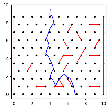
Next week, Marika and I will be flying to Massachusetts to visit my parents, and receive the generous gift of their camper van! Our trip happens to overlap which a favorite event on my childhood, the Ashfield Fall Festival. It includes local art, music, and cooking, but I was always more interested in the games. There was the usual tipping ladder, but my game of choice was the marble rolls. These were made from boards tipped at an angle with a grid of nails pounded into them. Rubber bands were stretched between nails in a pattern so that a marble dropped from the top would bounce off the nails and bands until it landed in one of the slots at the bottom. Different slots were worth different points that would determine your prize. I've now been studying physics for half my life, so I thought I could look at the game not as lottery, but as a deterministic physical system, and maybe win myself some grand-prize trinkets on this trip!

As the marble rolls down, it hits nails and bands that change its direction. Physicists typically look at collisions from two extremes: elastic and inelastic collisions. In both cases, momentum is conserved. For elastic collisions, energy is also conserved, but inelastic collisions in which the objects "hit and stick," or finish with the same velocity, lose the most energy possible while maintaining momentum conservation. For collisions between our marble and the nails/bands, the velocity we care about is only in the direction connecting the two objects: both collisions will stop the marble from going through it, but keep the component of velocity perpendicular the same. For nails we'll use inelastic collisions, which simply stop any motion through the nail, and for rubber bands we'll use elastic collisions, which reverse the direction.

I wrote some Python code to simulate this, randomly choosing pairs of adjacent nails to stretch bands between. Checking when the marble hits a nail is pretty simple, since we can just get the distance between the points and see if it's within the radius of the marble. The bands are a bit more involved: we have a line segment between two points, and need to know the distance to a third point. The closest point on the line segment will be on the perpendicular that passes through the marble's center (proof left as an exercise for the reader, heh). I ran into a couple edge effects in the simulation, where the marble would get sort of "hooked" on one of the nails, but overall I'm pleased with the results:

Now that we have this basic framework, we can generate a board, then map out the landing positions for all the different starting points. I decided to make a sort of flip-book with different numbers of bands, randomly chosen. The starting positions are shown by different colored lines, and the bottom of the plot shows a histogram of where the marbles land.

I couldn't figure out a good way to get statistical measures, but it's interesting to see the gaps just below bands where no marbles pass through, and to see cases where a marble starting on one side of the board crosses to the other side. The 0-band case has a nice symmetry to it, and some of the middle ones look a bit like Jackson Pollock paintings, but the important part is, with this on my side, that plastic lobster harmonica is mine!

On My Soapbox

I've been applying to a bunch of faculty positions recently, and one requested a recorded teaching sample. I made this, giving an introduction to special relativity. Questions & feedback are welcome!

Mixed Signals

Recently for my research I've been working with digital signal filters, which are a way to change the frequencies that appear in a signal. Specifically, I've been using a Kaiser bandpass filter, which removes frequencies outside a given range. You might imagine that if we want a specific range of frequencies, we could just use a Fourier transform to set those points to zero. There's a problem with that though: In order for the transform to be precise, we need infinitely long data, so we can capture all frequencies. Since ours is finite, we will get spectral leakage, where the timespan of our data will introduce its own frequency to the spectrum. We can mitigate this by applying a window to the data, which tapers at the ends.

These filters are often displayed through their finite impulse response (FIR), which shows what the filter does to a single spike of signal. Below are responses for a square window, which corresponds to the sharp clipping I described above, and an example Kaiser window:

Notice that the square window has much more wiggling on the sides, while the Kaiser window damps out quickly. On the other hand, we do lose a little bit of power in the main lobe of the Kaiser – There are always tradeoffs in these situations.

Once we have the FIR for a filter, we can apply it to a signal with an operation called convolution:

You can picture this as sliding the filter across the signal and taking the sum of the product at each point – The Wikipedia article I linked has some nice animations. What I wanted to know was, how do the different settings for the Kaiser filter affect the result for the signals I'm working on? Below, you'll find a plot of a square pulse before and after filtering. The controls are the attenuation outside the band of desired frequencies, the width of desired frequencies, and the cutoff, which is related to how long the transition from the passed to the attenuated frequencies lasts.