Flying First Class

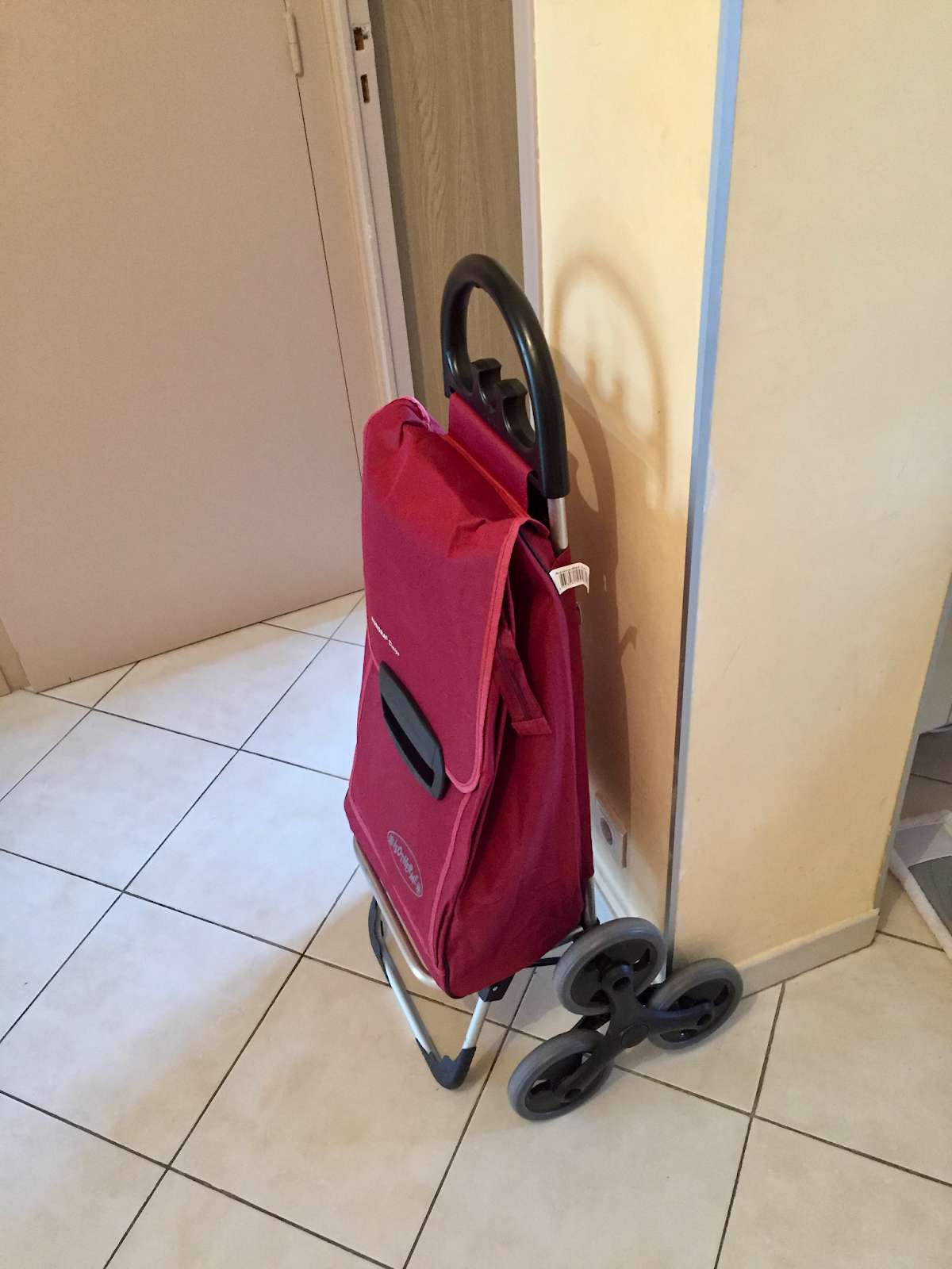
In a little more than a week, I'll be joined in France by Marika and Lorna! This weekend I decided to pick up some supplies, like dog food and more bedding, and I was all over town yesterday. Most places are closed on Sundays here, so I was glad to have a nice rolling cart to carry everything at once:

Notice the three wheels arranged in a triangle – This allows the bag to to climb stairs, a helpful feature when you live 3 flights up! The three wheels rotate when the front one hits the face of a step:

I was curious how much this reduced the force that needed to be applied to climb the stairs. We can consider one step as the center joint rotating around the front wheel:

F is the force applied to the handle at an angle φ from the horizontal, and mg is the force of gravity pointing down. These each apply a torque to the joint:

where r is the length of the spokes. To climb a step, the wheels rotate 120° around the joint so the upper wheel lands on the next step. The question is, what are the values of θ that the wheel rotates through? We can simplify things if we make φ match the slope of the stairs. Then, after a bit of geometry that gave me middle-school flashbacks, we have that θ is in the range

If we apply just enough force to overcome gravity (𝛕 = 0), the force is

We can plot this for a couple different slopes:

The vertical lines represent the starting θ, and then you follow the curve to zero. The slopes are 15° in red, 37.5° in blue, and 52.5° in green. I think there must be a mistake in this model, since more vertical slopes require less force, even though a straight lift requires a force of 1 on this scale, the dotted line. Despite the effort saved by this invention, I'm still too worn out to find my error!

Generalized Liquid Undulation Grapher (GLUG!)

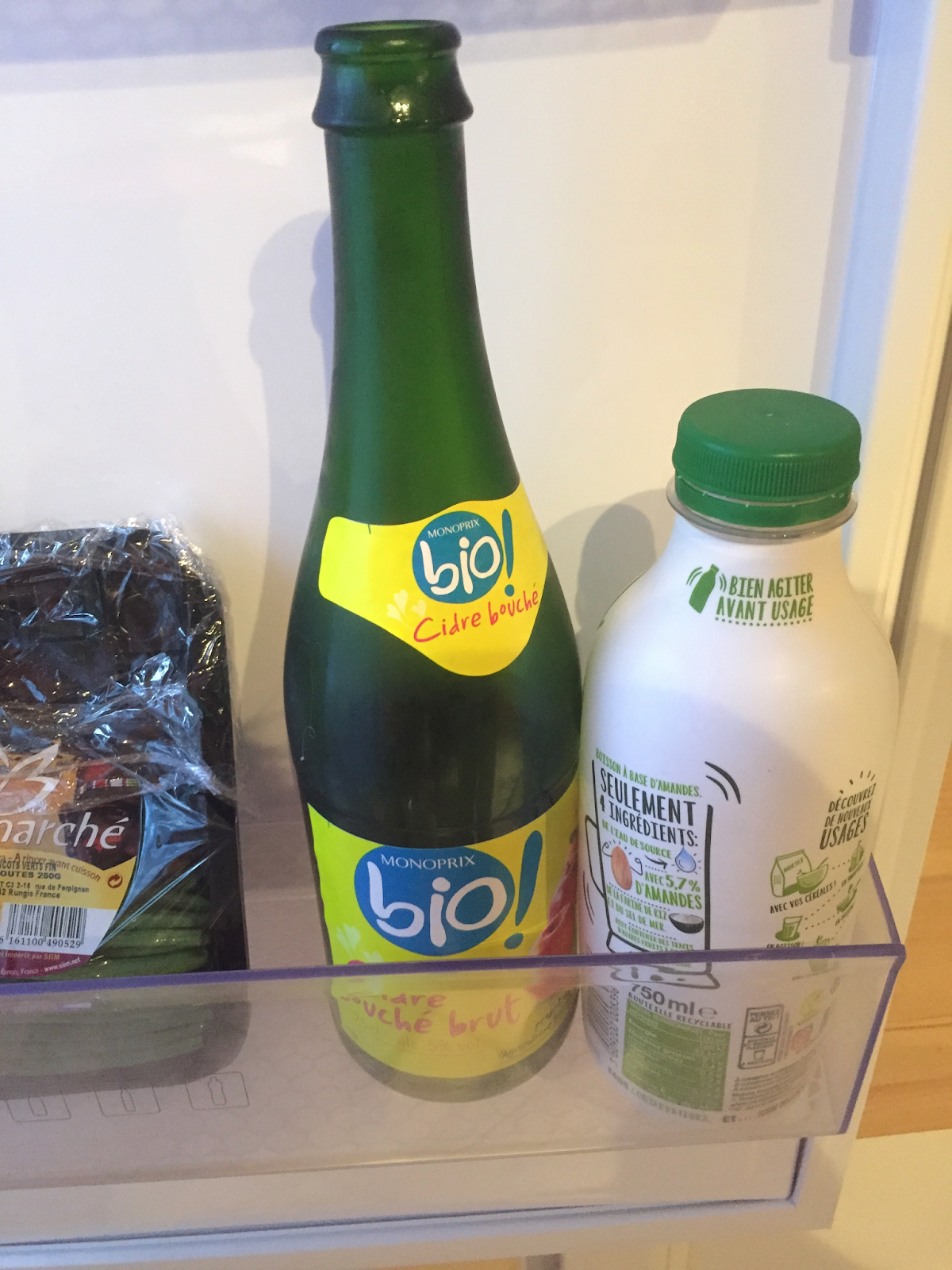
It seems here in France they only sell whole and 2% milk, no skim, so I've been relying on almond/soy milk for my morning coffee. Trouble is, those come in a container style that causes me no end of irritation:

The spout is so tiny that the liquid blocks it, causing the system to oscillate between pouring out liquid and sucking in air. This is especially bad when the container is nearly full, and I usually wind up spilling some.

To try to get something good out of this bad design, I wondered if I could predict what the rate of oscillation is between the two states. I figured I'd simplify things a bit, and just consider the bottle completely upside down:

We have a volume of air, a volume of liquid, an inner diameter D, and an opening diameter d. This situation is similar to that of an orifice plate, which uses Bernoulli's principle to determine the mass flow rate through an opening:

C_d is a constant called the coefficient of discharge, which depends on the shape of the opening, 𝜌 is the density of the liquid, and Δp is the difference in pressure across the opening. The air pressure inside starts off at normal atmospheric pressure when the bottle is right-side up, but as the liquid runs out, the volume of the air increases, proportionally decreasing the pressure:

The other pressure inside the bottle is the weight of the liquid:

For the flow equation, we want the difference between these two pressures and the outside air pressure, p_0. We can switch the mass flow from above to a volume using the density, which gives a differential equation once we plug everything in:

This is a mess, and when I tried to put some real numbers in, I realized the weight term is orders of magnitude smaller than the other pressures – This makes sense looking at the video, since each "glug" is only a small amount of liquid. More enlightening might be to find the amount of liquid that pours before the pressures are equal. Setting the terms under the radical to zero gives 8.7 microliters, which makes me less sure of my "this makes sense" assertion above. Either I've made an algebraic error, or (more charitably) this is not an accurate model of the system. I suppose I'll just have to add this to the collection of unsatisfying results!

Virulent Voronoi

This week, I was reading some background for my research, and I learned about something called a Voronoi pattern, which caught my attention. The basic idea is that for a set of points, you divide space into cells based on which point they're closest to. It's connected to my research because we compare incoming signals to a finite set of templates. When we say a particular template is the closest match for a signal, we want to know how far away it could be, i.e. the space spanned by that template.

Voronoi patterns appear in nature frequently – One way to make the pattern for a set of points is to expand each point in a circle, until they collide, which is exactly what would happen if you put several bacterial cultures in a Petri dish. Pixar animators use them to design scale patterns and other natural formations:

What interested me was using different measures of distance, not just the Euclidean distance to find the "closest" point. I wrote up a Python script to make these plots for a set of points, and a given distance measure. There are some really clever ways to make these diagrams, but I took a brute-force approach of dividing the space into a grid, and finding the nearest point for each box. For distance measures, I used the usual Euclidean distance, the metropolitan or taxi-cab metric, and the relativistic spacetime interval.

Euclidean Distance
This is the usual distance measure you probably learned in high school. A straight line between two points has a length of

For a random set of 5 points, we can divide a space into regions based on which point they're closest to.

Set 1, Euclidean

Set 2, Euclidean

Metropolitan Distance
You don't always want to measure distance with straight lines though. In a city, the streets are laid out in a grid, so you always have to move at right angles. In this case we just sum the vertical and horizontal differences:

 

For the same two sets of points, this gives some very different regions.

Set 1, Metropolitan

Set 2, Metropolitan

Spacetime Interval
In special relativity, there's a quantity called the spacetime interval, which gives properties of a path through spacetime. In this case, we usually work with the square:

Here c is the speed of light, which puts time and space into the same units. If this quantity is positive, the path is called time-like, and could describe a massive particle's motion. If it's negative, the path is called space-like, which means the two points can only be connected by faster than light motion. Relativity assumes this is impossible, so a space-like curve can't describe motion. Finally, if the interval is zero, it describes a beam of light, since Δx/Δt = c.

If we look for the minimum positive spacetime interval for each point, we can apply the idea of a Voronoi pattern to relativistic motion. First an example with just 2 points, to see what kind of patterns this creates.

Example Spacetime

Time is along the vertical axis, and x is horizontal. Each point projects a region above and below. If we think of the points as observers, the regions represent positions and times for which that point is the first to see what happened there (or for points ahead of the observer, the first place they are observed). White areas show events that no observer can witness.

Keeping all that in mind, we can look at the previous two point sets under this metric.

Set 1, Spacetime

Set 2, Spacetime

These are a bit of a mess, but it's an interesting way to look at the spacetime interval. In the second set, there are several narrow slivers due to the metric favoring light-like (45° diagonal) paths.

I'm not sure this is useful for anything aside from making interesting pictures, but that's good enough for me!

Bubble Trouble

To celebrate New Years this past week, I got myself a bottle of hard cider, fearing the looks I would get for buying cheap champagne in the country of its origin. Since I'm still outfitting my apartment here, I had no way to cork the bottle after opening, but I was impressed with how long it kept its carbonation in the refrigerator. I thought I'd look into some of the models for gas solubility at different temperatures to understand the contributing factors.

Carbonated drinks are so named because they consist of carbon dioxide dissolved in liquid. The bubbles you see (and taste) on opening a bottle are pockets of CO2 coming out of solution. The amount of CO2 that stays in solution is given by Henry's Law:

where p is the partial pressure of the gas outside the liquid, kH is a coefficient that changes with temperature, and c is the concentration of the dissolved gas. Partial pressure means the fraction of overall pressure due to the specific gas that's dissolved, in this case the amount of CO2 in the atmosphere. As with any model, we're making approximations here, like the assumption that the CO2 acts like an ideal gas, only interacting with itself.

We're trying to compare the amount of CO2 that stays in the cider when refrigerated and at room temperature, so we need to look at how kH varies:

where k0 is kH at reference temperature T0, and C is a constant that depends on the gas being considered. The link above gives for CO2 at room temperature k0 = 29.41 L atm/mol, C = 2400 K, and T0 = 298 K. A typical temperature for refrigerators is 40°F or 277.6 K. Plugging these in, we find that kH will be about 55% smaller in the refrigerator. Since the partial pressure is the same inside and out, that means the concentration in the refrigerator is 1/0.55 = 80% larger than at room temperature.

When I started looking into this, I thought I would be finding a time it took to lose a given amount of carbonation, and the process would be slower in the fridge, but this model suggests that the carbonation will stay indefinitely. I think that's because even though having the CO2 outside the liquid is a lower-energy state overall, it takes some energy to create the bubbles – That's why shaking a soda makes it fizz. Happy New Year!